---
title: "Process Input Data for Models"
author: "Dave Bosworth"
date: today
date-format: long
format:
html:
toc: true
code-fold: show
code-tools: true
execute:
message: false
warning: false
---
# Purpose
Prepare input data for models used in the DWR nutrient synthesis project.
# Global Code
```{r load packages}
# Load packages
library(tidyverse)
library(readxl)
library(rlang)
library(glue)
library(hms)
library(scales)
library(sf)
library(mapview)
library(EDIutils)
library(fs)
library(here)
library(conflicted)

# Declare package conflict preferences
conflicts_prefer(dplyr::filter(), hms::hms())
```
```{r session info}
# Run session info to display package versions
devtools::session_info()
```
Create functions used in this document:
```{r functions}
# Get data entity names for specified EDI ID
get_edi_data_entities <- function(edi_id) {
  df_data_ent <- read_data_entity_names(edi_id)
  inform(c(
    "i" = paste0(
      "Data entities for ",
      edi_id,
      " include:\n",
      paste(df_data_ent$entityName, collapse = "\n"),
      "\n"
    )
  ))
  return(df_data_ent$entityName)
}

# Download specified data entities from an EDI package and save raw bytes files to a
# temporary directory
get_edi_data <- function(edi_id, entity_names) {
  df_data_ent <- read_data_entity_names(edi_id)
  df_data_ent_filt <- df_data_ent %>% filter(entityName %in% entity_names)

  ls_data_raw <-
    map(df_data_ent_filt$entityId, \(x) {
      read_data_entity(edi_id, entityId = x)
    }) %>%
    set_names(df_data_ent_filt$entityName)

  temp_dir <- tempdir()
  for (i in 1:length(ls_data_raw)) {
    file_raw <- file.path(temp_dir, glue("{names(ls_data_raw)[i]}.bin"))
    con <- file(file_raw, "wb")
    writeBin(ls_data_raw[[i]], con)
    close(con)
  }
}

# Replace values below the reporting limit with simulated values between `min_val`
# and the RL
replace_blw_rl <- function(df, min_val = 0, seed = 1) {
  # Pull out values that are below the RL
  df_blw_rl <- df %>% filter(Sign == "<")

  # Replace below RL values with simulated ones
  withr::with_seed(
    # Set seed for reproducibility
    seed = seed,
    df_blw_rl_sim <- df_blw_rl %>%
      mutate(
        Result = round(runif(nrow(df_blw_rl), min = min_val, max = Result), 6)
      )
  )

  # Add simulated values back to main data frame
  df %>% filter(Sign != "<") %>% bind_rows(df_blw_rl_sim)
}

# Add variable for season as a factor
add_season <- function(df) {
  df %>%
    mutate(
      Season = case_match(
        Month,
        3:5 ~ "Spring",
        6:8 ~ "Summer",
        9:11 ~ "Fall",
        c(12, 1, 2) ~ "Winter"
      ),
      Season = factor(Season, levels = c("Winter", "Spring", "Summer", "Fall"))
    )
}
```
Load globally-used data:
```{r load global data}
# Load regions shapefile
sf_delta <- read_sf(here("data/spatial/delta_subregions.shp"))
```
# Regions Map
Create map showing SubRegions and Regions used to process the data.
```{r}
mapview(sf_delta, zcol = "Region", alpha.regions = 0.5)
```
# DWR Integrated Discrete Nutrient Data
## Import Data
```{r dwr nutr import data}
# Import nutrient data set
df_nutr <- readRDS(here("data/processed/nutrient_data_discrete.rds"))

# Import phytoplankton data from FRP's EDI publication to assign lat-long coordinates
# to FRP's nutrient data in the DWR integrated discrete nutrient data set
edi_id_frp <- "edi.269.5"
edi_data_ent_frp <- get_edi_data_entities(edi_id_frp)
edi_data_ent_frp_phyto <- str_subset(edi_data_ent_frp, "^phyto")
get_edi_data(edi_id_frp, edi_data_ent_frp_phyto)
temp_files <- list.files(tempdir(), full.names = TRUE)

df_frp_phyto_coord <-
  read_csv(str_subset(temp_files, edi_data_ent_frp_phyto)) %>%
  drop_na(LatitudeStart, LongitudeStart) %>%
  summarize(
    Latitude = mean(LatitudeStart),
    Longitude = mean(LongitudeStart),
    .by = Location
  )
```
## Prepare Data
```{r dwr nutr prepare data}
# Prepare data for aggregation
df_nutr_c1 <- df_nutr %>%
  # Add lat-long coordinates for FRP stations from the phytoplankton data set
  filter(Project == "Fish Restoration Program") %>%
  select(-c(Latitude, Longitude)) %>%
  left_join(df_frp_phyto_coord, by = join_by(Station_Name == Location)) %>%
  bind_rows(df_nutr %>% filter(Project != "Fish Restoration Program")) %>%
  # Remove records without lat-long coordinates
  drop_na(Latitude, Longitude) %>%
  # Assign SubRegions to the stations
  st_as_sf(coords = c("Longitude", "Latitude"), crs = 4326) %>%
  st_transform(crs = st_crs(sf_delta)) %>%
  st_join(sf_delta, join = st_intersects) %>%
  # Remove any data outside our subregions of interest
  filter(!is.na(SubRegion)) %>%
  st_drop_geometry()
```
Remove various duplicated records so that there is only one sample per station-day.
```{r dwr nutr rm dt dups}
# Clean up duplicated records that share same Date_Time - it might be more
# appropriate to address this in the nutrient data integration code. TODO: talk to
# Morgan about this
df_nutr_dt_dups <- df_nutr_c1 %>%
  add_count(Project, Station_Name, Date_Time, Analyte) %>%
  filter(n > 1) %>%
  select(-n) %>%
  drop_na(Date_Time)

# Keep the records with the "earliest" Sample_Code
df_nutr_dt_dups_fixed <- df_nutr_dt_dups %>%
  arrange(Project, Station_Name, Date_Time, Analyte, Sample_Code) %>%
  distinct(Project, Station_Name, Date_Time, Analyte, .keep_all = TRUE)

df_nutr_c2 <- df_nutr_c1 %>%
  anti_join(df_nutr_dt_dups) %>%
  bind_rows(df_nutr_dt_dups_fixed)
```
```{r dwr nutr rm dups no dt}
# Clean up duplicated records that share same Date and don't have a collection time
df_nutr_dups_nodt <- df_nutr_c2 %>%
  add_count(Project, Station_Name, Date, Analyte) %>%
  filter(n > 1, is.na(Date_Time)) %>%
  select(-n)

# Keep the records with the "earliest" Sample_Code
df_nutr_dups_nodt_fixed <- df_nutr_dups_nodt %>%
  arrange(Project, Station_Name, Date, Analyte, Sample_Code) %>%
  distinct(Project, Station_Name, Date, Analyte, .keep_all = TRUE)

df_nutr_c3 <- df_nutr_c2 %>%
  anti_join(df_nutr_dups_nodt) %>%
  bind_rows(df_nutr_dups_nodt_fixed)
```
```{r dwr nutr rm dups same day}
# Filter data so that there is only one sample per station-day by choosing the data
# point closest to noon
df_nutr_daily_dups <- df_nutr_c3 %>%
  add_count(Project, Station_Name, Date, Analyte) %>%
  filter(n > 1) %>%
  select(-n)

df_nutr_daily_dups_fixed <- df_nutr_daily_dups %>%
  # Create variable for time and calculate difference from noon for each data point
  mutate(
    Time = as_hms(Date_Time),
    Noon_diff = abs(hms(hours = 12) - Time)
  ) %>%
  group_by(Project, Station_Name, Date, Analyte) %>%
  # Select only 1 data point per Station, Date, and Analyte, choose data closest to
  # noon
  filter(Noon_diff == min(Noon_diff)) %>%
  # When points are equidistant from noon, select earlier point
  filter(Time == min(Time)) %>%
  ungroup() %>%
  select(-c(Time, Noon_diff))

df_nutr_c4 <- df_nutr_c3 %>%
  anti_join(df_nutr_daily_dups) %>%
  bind_rows(df_nutr_daily_dups_fixed)
```
Replace values below the reporting limit with simulated values.
```{r dwr nutr replace blw rl vals}
# Replace values below the reporting limit with simulated values
df_nutr_c5 <- df_nutr_c4 %>%
  mutate(
    Sign = if_else(Detection_Condition == "Not Detected", "<", "="),
    Result = if_else(
      Detection_Condition == "Not Detected",
      Reporting_Limit,
      Result
    ),
    .keep = "unused"
  ) %>%
  # Omit <RL values with reporting limits that are greater than the 95th percentile
  # of the values for the parameter
  mutate(q95 = quantile(Result, probs = 0.95), .by = Analyte) %>%
  filter(!(Sign == "<" & Result > q95)) %>%
  select(-q95) %>%
  replace_blw_rl()
```
## Aggregate Data
```{r dwr nutr calc monthly values}
# Calculate Monthly-Regional averages
df_nutr_avg_mo <- df_nutr_c5 %>%
  mutate(
    Year = year(Date),
    Month = month(Date)
  ) %>%
  summarize(
    Result = mean(Result),
    Num_samples = n(),
    .by = c(Year, Month, Region, Analyte)
  )
```
```{r dwr nutr calc seasonal values}
# Further calculate Seasonal-Regional averages using Adjusted calendar year:
# December-November, with December of the previous calendar year included with the
# following year
df_nutr_avg_seas <- df_nutr_avg_mo %>%
  mutate(YearAdj = if_else(Month == 12, Year + 1, Year)) %>%
  add_season() %>%
  summarize(
    Result = mean(Result),
    Num_samples = sum(Num_samples),
    .by = c(YearAdj, Season, Region, Analyte)
  )
```
```{r dwr nutr conv monthly seasonal to wide}
# Convert both sets of averages to wide format
ls_nutr_avg_wide <- lst(df_nutr_avg_mo, df_nutr_avg_seas) %>%
  map(
    \(x) {
      mutate(
        x,
        Analyte = case_match(
          Analyte,
          "Dissolved Ammonia" ~ "DissAmmonia",
          "Dissolved Nitrate" ~ "DissNitrate",
          "Dissolved Nitrate + Nitrite" ~ "DissNitrateNitrite",
          "Dissolved Organic Nitrogen" ~ "DON",
          "Dissolved ortho-Phosphate" ~ "DissOrthophos",
          "Total Kjeldahl Nitrogen" ~ "TKN",
          "Total Phosphorus" ~ "TotPhos"
        )
      ) %>%
        arrange(Analyte, .locale = "en") %>%
        select(-Num_samples) %>%
        pivot_wider(names_from = Analyte, values_from = Result)
    }
  )
```
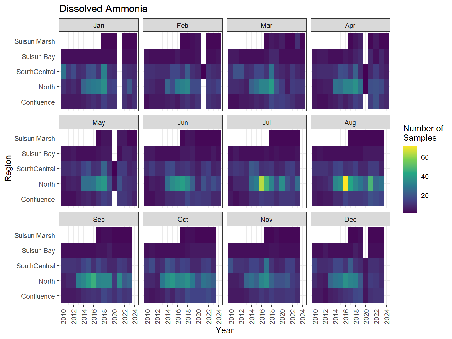
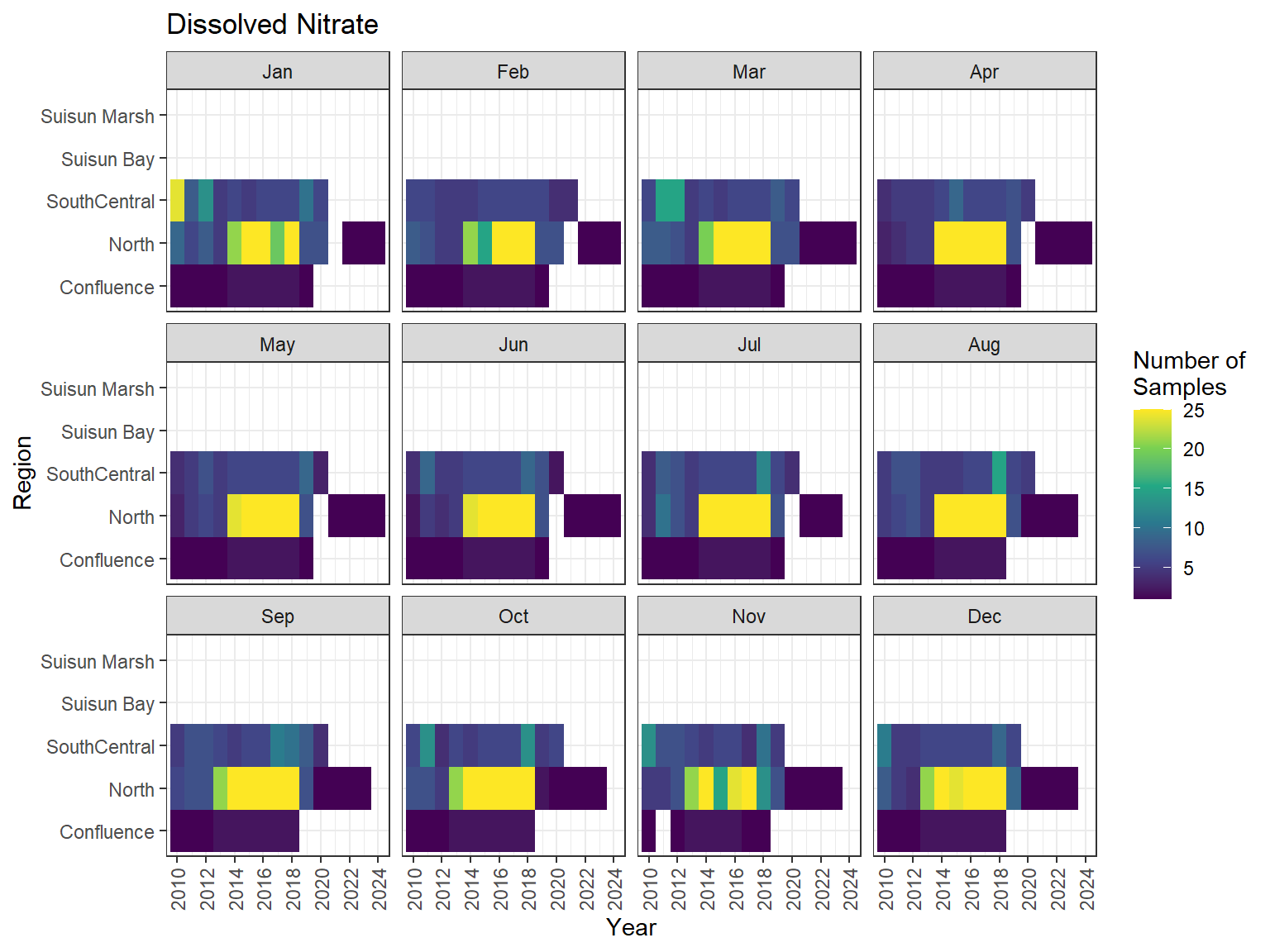
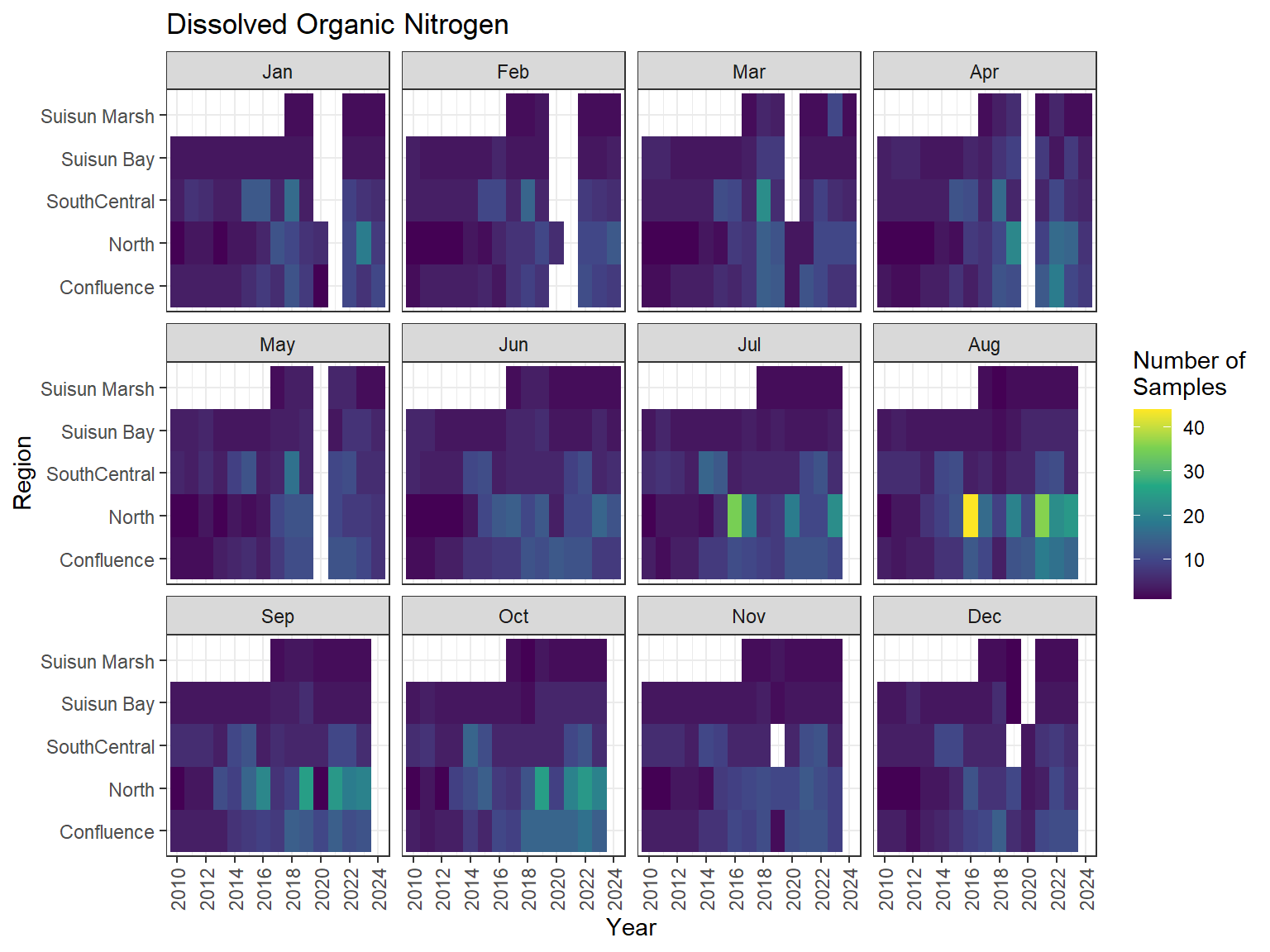
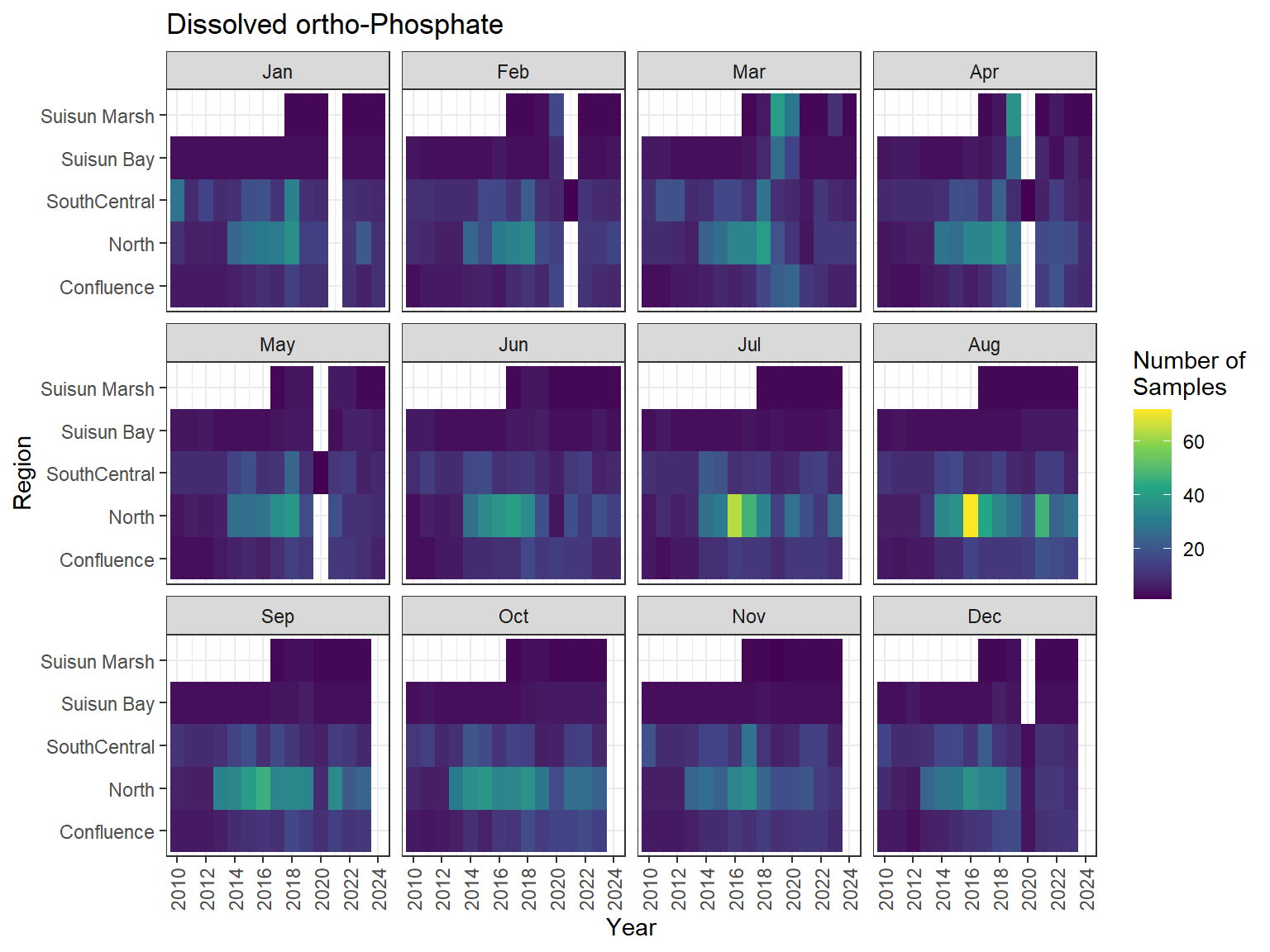
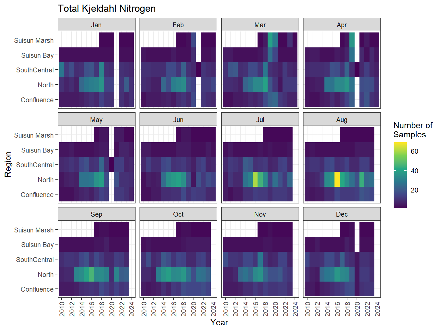
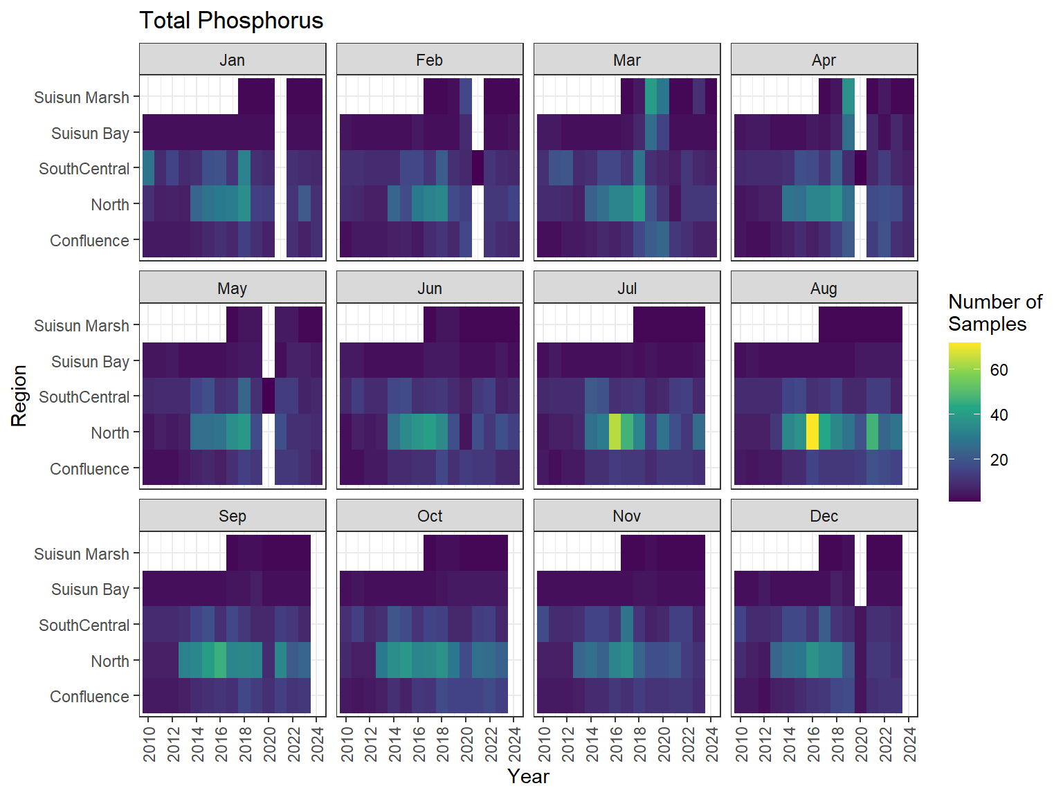
## Sampling Effort Plots
### Monthly Values
```{r dwr nutr samp effort monthly values}
ls_nutr_avg_mo_plt <- df_nutr_avg_mo %>%
  mutate(Month = month(Month, label = TRUE)) %>%
  complete(nesting(Year, Month), Region, Analyte) %>%
  nest(.by = Analyte) %>%
  deframe() %>%
  imap(
    \(x, idx) {
      ggplot(data = x, aes(x = Year, y = Region, fill = Num_samples)) +
        geom_tile() +
        facet_wrap(vars(Month)) +
        ggtitle(idx) +
        scale_y_discrete(drop = FALSE) +
        scale_x_continuous(
          breaks = breaks_pretty(10),
          expand = expansion(mult = 0.02)
        ) +
        scale_fill_viridis_c(
          name = "Number of\nSamples",
          na.value = "transparent"
        ) +
        theme_bw() +
        theme(axis.text.x = element_text(angle = 90, hjust = 1, vjust = 0.5))
    }
  )
```
::: {.panel-tabset}
```{r dwr nutr print samp effort monthly values}
#| echo: false
#| results: asis
#| fig-width: 8
#| fig-height: 6
for (i in 1:length(ls_nutr_avg_mo_plt)) {
# Create subheadings for each Parameter
cat("#### ", names(ls_nutr_avg_mo_plt[i]), "\n\n")
# Print plot
print(ls_nutr_avg_mo_plt[[i]])
cat("\n\n")
}
```
:::
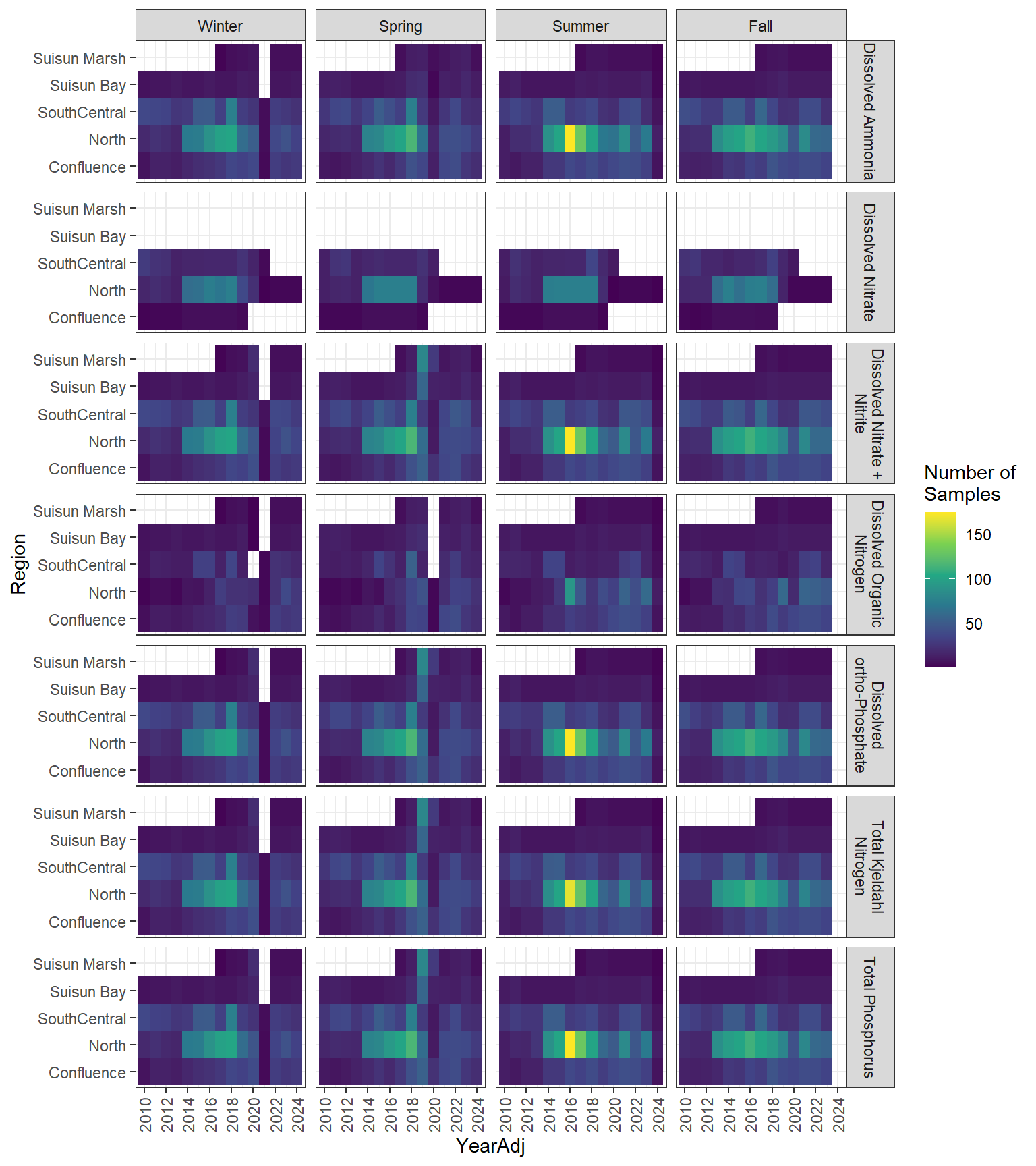
### Seasonal Values
```{r dwr nutr samp effort seasonal values}
#| fig-width: 8
#| fig-height: 9
df_nutr_avg_seas %>%
  ggplot(aes(x = YearAdj, y = Region, fill = Num_samples)) +
  geom_tile() +
  facet_grid(
    rows = vars(Analyte),
    cols = vars(Season),
    labeller = label_wrap_gen(width = 20)
  ) +
  scale_x_continuous(
    breaks = breaks_pretty(10),
    expand = expansion(mult = 0.02)
  ) +
  scale_fill_viridis_c(name = "Number of\nSamples") +
  theme_bw() +
  theme(axis.text.x = element_text(angle = 90, hjust = 1, vjust = 0.5))
```
# Integrated Discrete WQ Data from discretewq
## Import Data
```{r discretewq import data}
# Import integrated water quality data set from discretewq
df_dwq <- readRDS(here("data/external/discretewq_2009_2024.rds"))
```
## Prepare Data
```{r discretewq prepare data}
# Define water quality parameters to keep from discretewq
dwq_param <- c(
  "Microcystis",
  "Temperature",
  "Salinity",
  "DissolvedOxygen",
  "pH",
  "TurbidityNTU",
  "TurbidityFNU",
  "Chlorophyll"
)

# Prepare data for aggregation
df_dwq_c1 <- df_dwq %>%
  select(
    Source,
    Station,
    Latitude,
    Longitude,
    Date,
    Datetime,
    Year,
    Month,
    all_of(dwq_param),
    Chlorophyll_Sign
  ) %>%
  # Convert Datetime to PST
  mutate(Datetime = with_tz(Datetime, tzone = "Etc/GMT+8")) %>%
  # Remove rows where all parameters are NA
  filter(!if_all(all_of(dwq_param), is.na)) %>%
  # Remove records without lat-long coordinates
  drop_na(Latitude, Longitude) %>%
  # Assign SubRegions to the stations
  st_as_sf(coords = c("Longitude", "Latitude"), crs = 4326) %>%
  st_transform(crs = st_crs(sf_delta)) %>%
  st_join(sf_delta, join = st_intersects) %>%
  # Remove any data outside our subregions of interest
  filter(!is.na(SubRegion)) %>%
  st_drop_geometry() %>%
  # Only keep the stations located in Suisun, Montezuma, and Nurse Sloughs from the
  # Suisun Marsh survey
  filter(!(Source == "Suisun" & !str_detect(Station, "^SU|^MZ|^NS")))

# Pivot the parameter columns to long data structure
df_dwq_c2 <- df_dwq_c1 %>%
  # Add a value suffix to the parameter columns
  rename_with(\(x) paste0(x, "_Result"), all_of(dwq_param)) %>%
  # Pivot parameters longer, creating a sign and result column for each parameter
  pivot_longer(
    cols = ends_with(c("Sign", "Result")),
    names_to = c("Parameter", ".value"),
    names_pattern = "(.*)_(.*)"
  ) %>%
  drop_na(Result) %>%
  replace_na(list(Sign = "="))
```
Consolidate Turbidity parameters and prefer TurbidityNTU when both NTU and FNU were collected.
```{r discretewq consolidate turbidity}
df_dwq_c3 <- df_dwq_c2 %>%
  mutate(
    Parameter2 = if_else(
      str_detect(Parameter, "^Turbidity"),
      "Turbidity",
      Parameter
    )
  )

df_dwq_turb_dups <- df_dwq_c3 %>%
  filter(Parameter2 == "Turbidity") %>%
  add_count(Source, Station, Datetime) %>%
  filter(n > 1) %>%
  select(-n)

df_dwq_turb_dups_fixed <- df_dwq_turb_dups %>%
  filter(Parameter == "TurbidityNTU")

df_dwq_c4 <- df_dwq_c3 %>%
  anti_join(df_dwq_turb_dups) %>%
  bind_rows(df_dwq_turb_dups_fixed) %>%
  select(-Parameter) %>%
  rename(Parameter = Parameter2)
```
Remove various duplicated records so that there is only one sample per station-day.
```{r discretewq rm dt dups}
# Clean up the duplicated records that share same Datetime from EDSM
df_dwq_dt_dups <- df_dwq_c4 %>%
  add_count(Source, Station, Datetime, Parameter) %>%
  filter(n > 1) %>%
  select(-n)

df_dwq_dt_dups_fixed <- df_dwq_dt_dups %>%
  distinct(Source, Station, Datetime, Parameter, .keep_all = TRUE)

df_dwq_c5 <- df_dwq_c4 %>%
  anti_join(df_dwq_dt_dups) %>%
  bind_rows(df_dwq_dt_dups_fixed)
```
```{r discretewq rm dups same day}
# Filter data so that there is only one sample per station-day by choosing the data
# point closest to noon
df_dwq_daily_dups <- df_dwq_c5 %>%
  add_count(Source, Station, Date, Parameter) %>%
  filter(n > 1) %>%
  select(-n)

df_dwq_daily_dups_fixed <- df_dwq_daily_dups %>%
  # Create variable for time and calculate difference from noon for each data point
  mutate(
    Time = as_hms(Datetime),
    Noon_diff = abs(hms(hours = 12) - Time)
  ) %>%
  group_by(Source, Station, Date, Parameter) %>%
  # Select only 1 data point per Station, Date, and Parameter, choose data closest to
  # noon
  filter(Noon_diff == min(Noon_diff)) %>%
  # When points are equidistant from noon, select earlier point
  filter(Time == min(Time)) %>%
  ungroup() %>%
  select(-c(Time, Noon_diff))

df_dwq_c6 <- df_dwq_c5 %>%
  anti_join(df_dwq_daily_dups) %>%
  bind_rows(df_dwq_daily_dups_fixed)
```
Remove values that are out of range of reasonable limits for the parameter
```{r discretewq rm outliers}
df_dwq_c7 <- df_dwq_c6 %>%
  # Temperature value of 2.9 collected on 8/12/2014 in Suisun Marsh
  filter(!(Parameter == "Temperature" & Result < 3)) %>%
  # Temperature value of 116 collected on 3/23/2017 at USGS-11447650
  filter(!(Parameter == "Temperature" & Result > 35)) %>%
  # DO values greater than 20 (these are obviously % Saturation)
  filter(!(Parameter == "DissolvedOxygen" & Result > 20)) %>%
  # pH value of 2.56 collected on 7/2/2014 in the Yolo Bypass
  filter(!(Parameter == "pH" & Result < 3)) %>%
  # Two Turbidity values greater than 1000 collected in early Sept 2017 in the South
  # Delta
  filter(!(Parameter == "Turbidity" & Result > 1000)) %>%
  # A few Chlorophyll values less than or equal to zero
  filter(!(Parameter == "Chlorophyll" & Result <= 0))
```
## Aggregate Data
```{r discretewq calc monthly values}
# Calculate Monthly-Regional averages
df_dwq_avg_mo <- df_dwq_c7 %>%
  # Convert pH values to H+ concentration before averaging
  mutate(Result = if_else(Parameter == "pH", 10^-Result, Result)) %>%
  # Replace Chlorophyll values below the reporting limit with simulated values
  replace_blw_rl() %>%
  summarize(
    Result = mean(Result),
    Num_samples = n(),
    .by = c(Year, Month, Region, Parameter)
  )
```
```{r discretewq calc seasonal values}
# Further calculate Seasonal-Regional averages using Adjusted calendar year:
# December-November, with December of the previous calendar year included with the
# following year
df_dwq_avg_seas <- df_dwq_avg_mo %>%
  mutate(YearAdj = if_else(Month == 12, Year + 1, Year)) %>%
  add_season() %>%
  summarize(
    Result = mean(Result),
    Num_samples = sum(Num_samples),
    .by = c(YearAdj, Season, Region, Parameter)
  )
```
```{r discretewq conv monthly seasonal to wide}
# Convert both sets of averages to wide format
ls_dwq_avg_wide <- lst(df_dwq_avg_mo, df_dwq_avg_seas) %>%
  map(
    \(x) {
      select(x, -Num_samples) %>%
        pivot_wider(names_from = Parameter, values_from = Result) %>%
        mutate(
          # Round Microcystis to nearest whole number
          Microcystis_round = round(Microcystis),
          # Convert average H+ concentration to average pH
          pH = -log10(pH)
        )
    }
  )
```
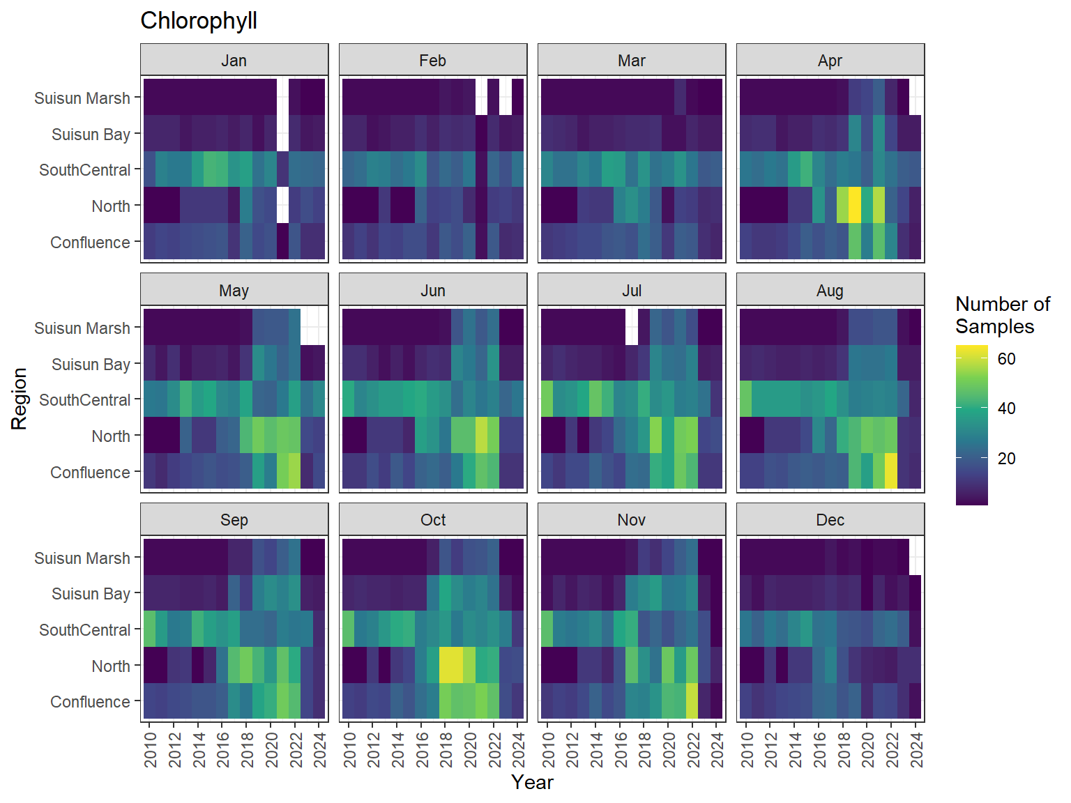
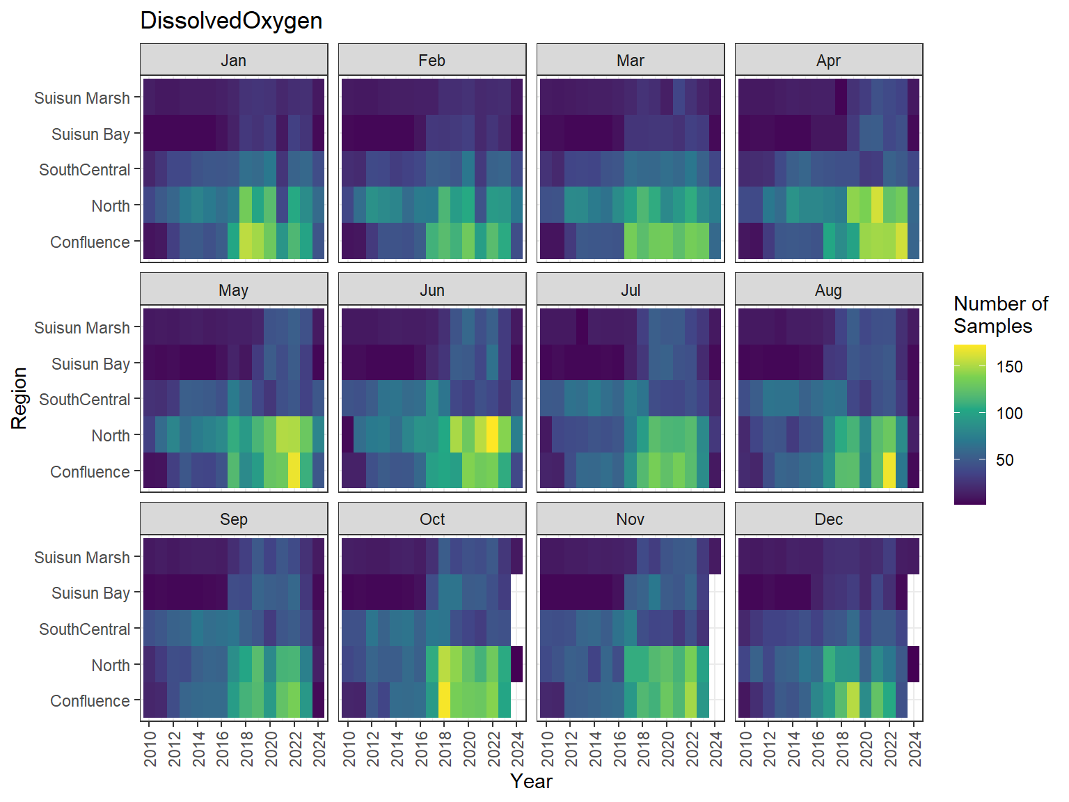
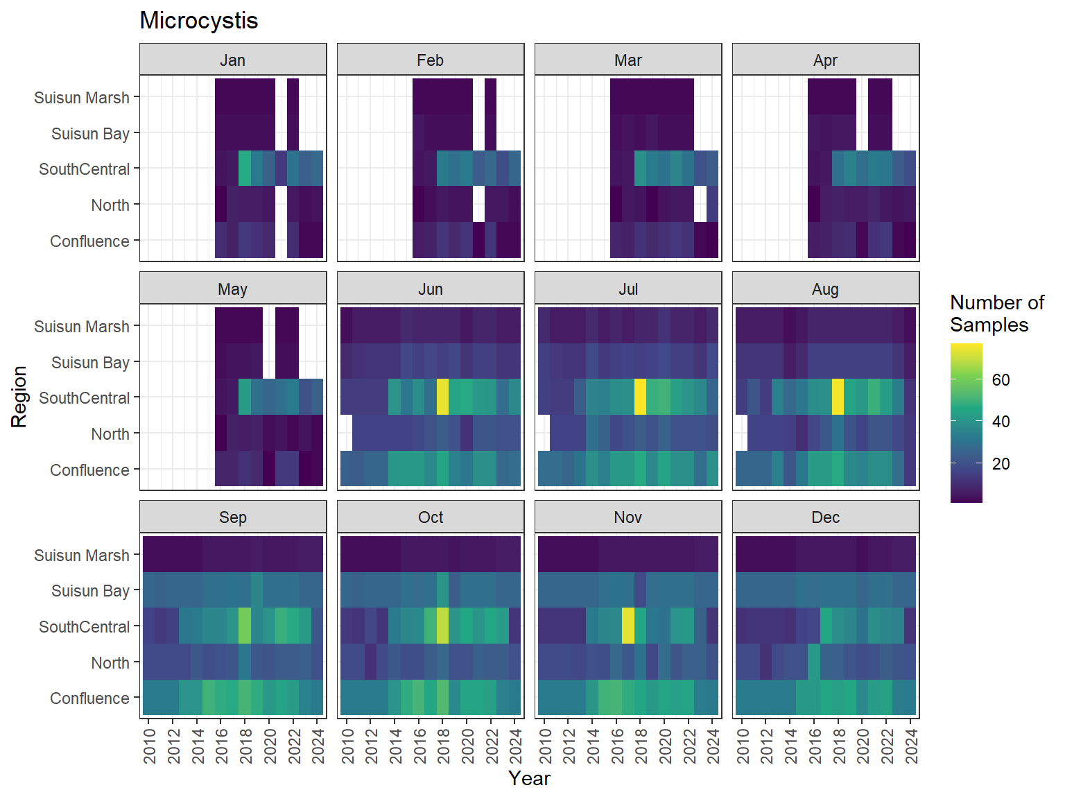
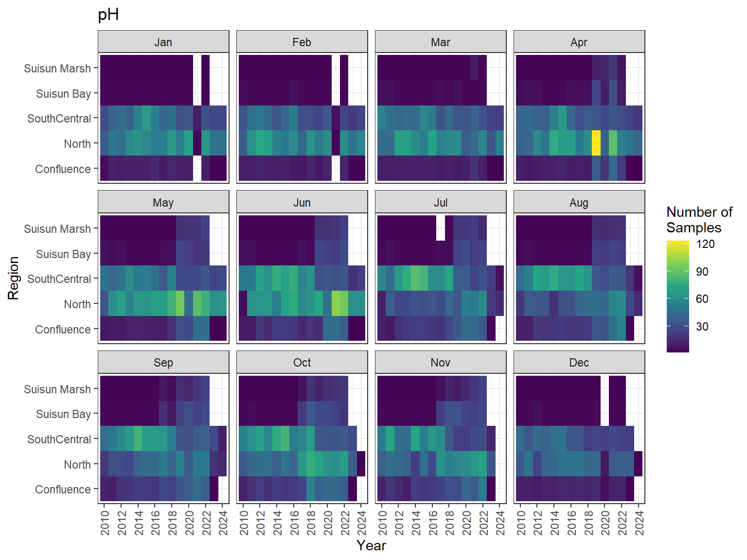
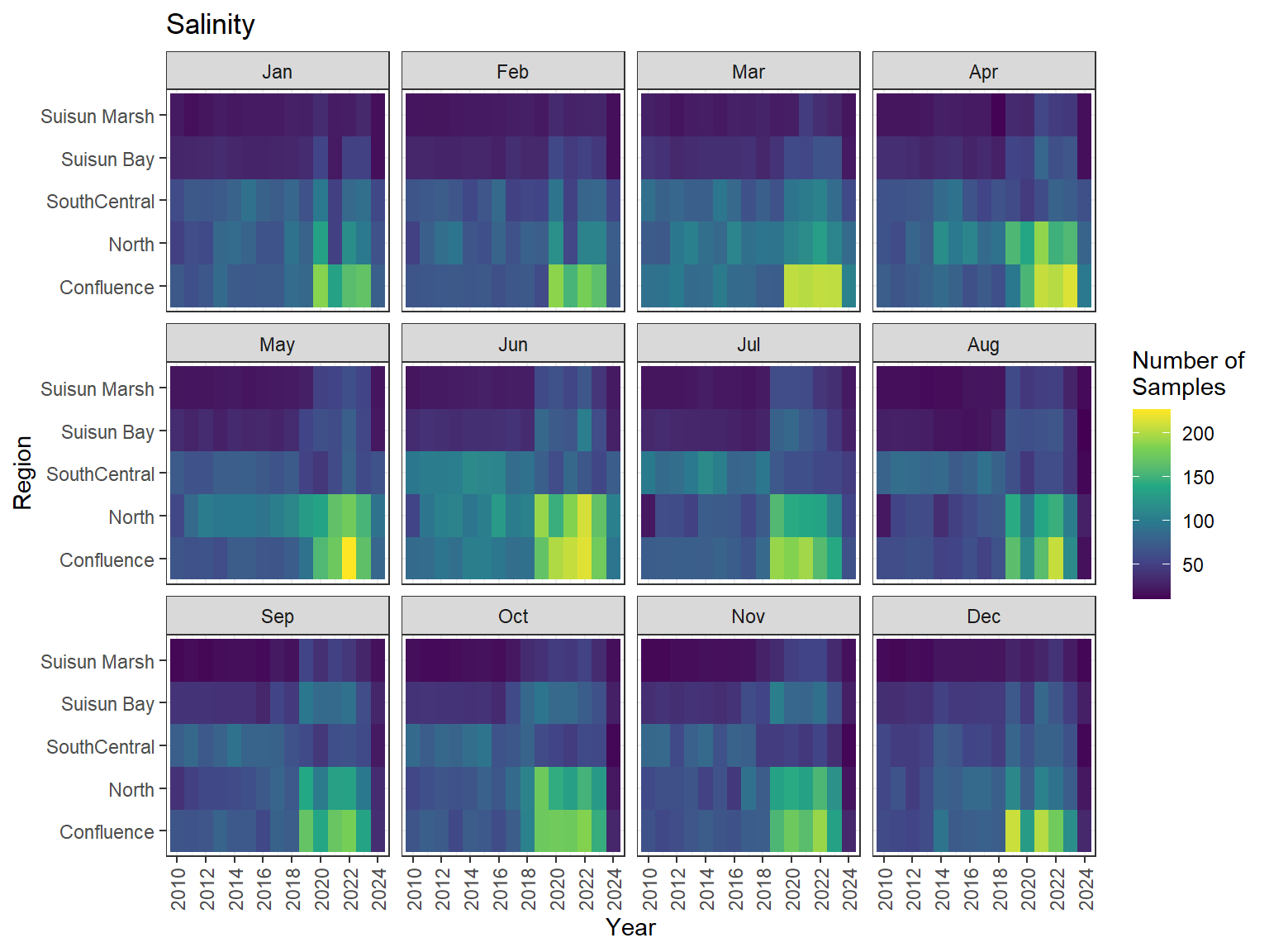
## Sampling Effort Plots
### Monthly Values
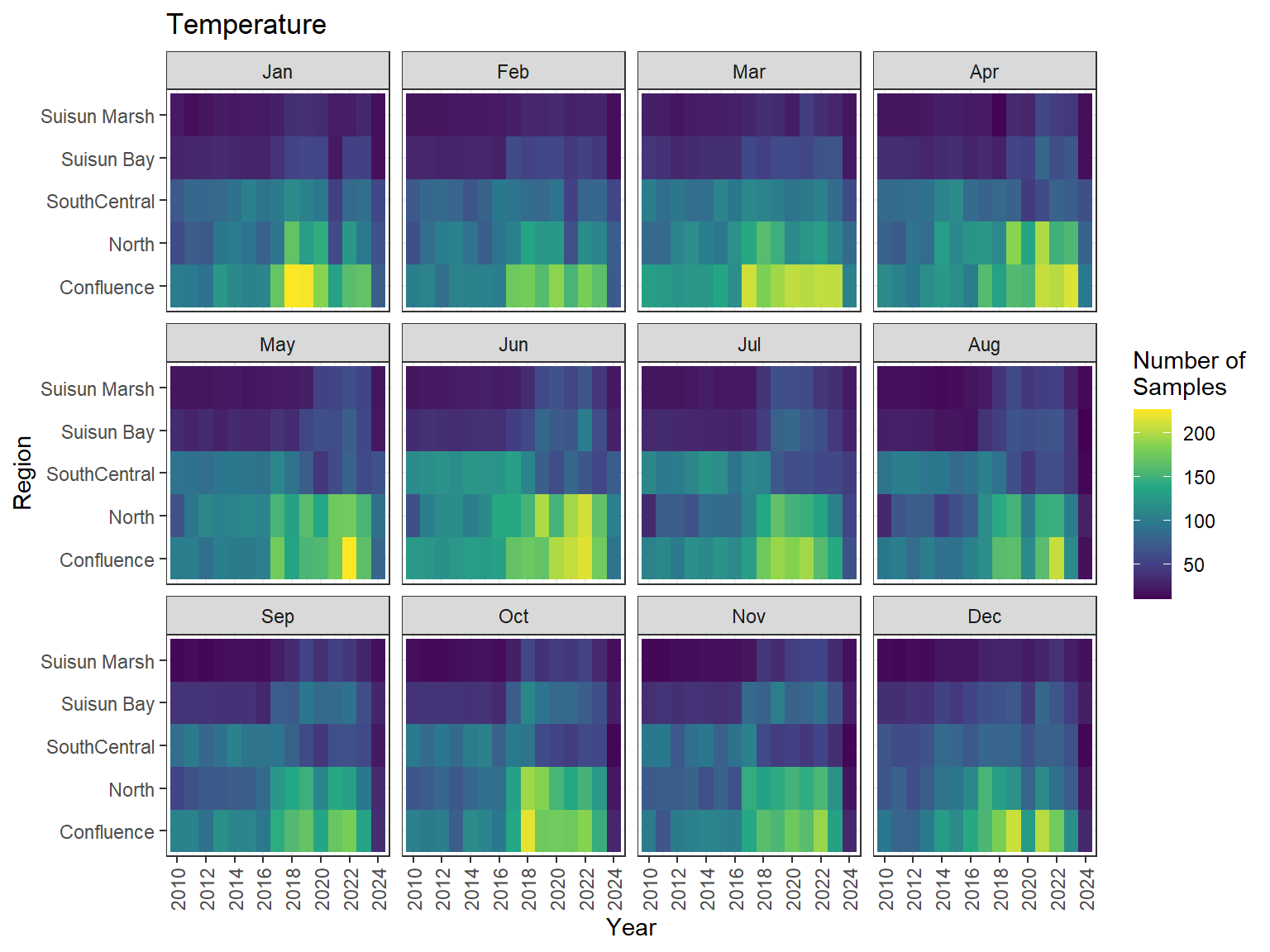
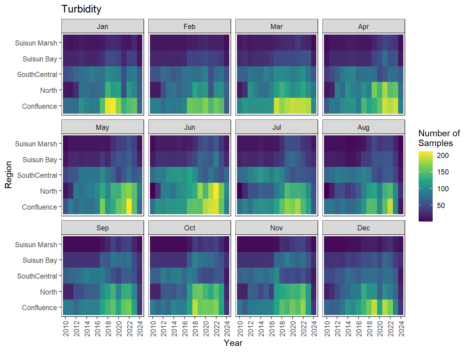
```{r discretewq samp effort monthly values}
ls_dwq_avg_mo_plt <- df_dwq_avg_mo %>%
  filter(Year %in% 2010:2024) %>%
  mutate(Month = month(Month, label = TRUE)) %>%
  complete(nesting(Year, Month), Region, Parameter) %>%
  nest(.by = Parameter) %>%
  deframe() %>%
  imap(
    \(x, idx) {
      ggplot(data = x, aes(x = Year, y = Region, fill = Num_samples)) +
        geom_tile() +
        facet_wrap(vars(Month)) +
        ggtitle(idx) +
        scale_y_discrete(drop = FALSE) +
        scale_x_continuous(
          breaks = breaks_pretty(10),
          expand = expansion(mult = 0.02)
        ) +
        scale_fill_viridis_c(
          name = "Number of\nSamples",
          na.value = "transparent"
        ) +
        theme_bw() +
        theme(axis.text.x = element_text(angle = 90, hjust = 1, vjust = 0.5))
    }
  )
```
::: {.panel-tabset}
```{r discretewq print samp effort monthly values}
#| echo: false
#| results: asis
#| fig-width: 8
#| fig-height: 6
for (i in 1:length(ls_dwq_avg_mo_plt)) {
# Create subheadings for each Parameter
cat("#### ", names(ls_dwq_avg_mo_plt[i]), "\n\n")
# Print plot
print(ls_dwq_avg_mo_plt[[i]])
cat("\n\n")
}
```
:::
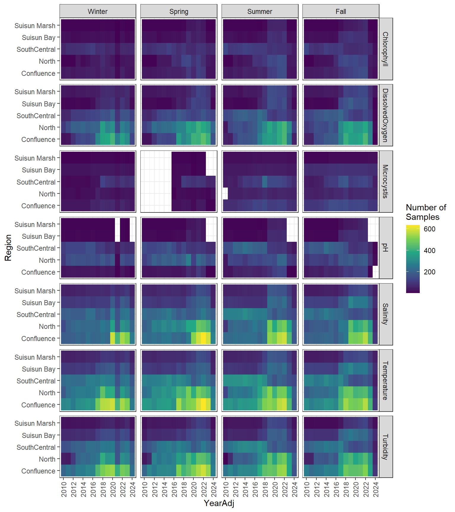
### Seasonal Values
```{r discretewq samp effort seasonal values}
#| fig-width: 8
#| fig-height: 9
df_dwq_avg_seas %>%
  filter(YearAdj %in% 2010:2024) %>%
  ggplot(aes(x = YearAdj, y = Region, fill = Num_samples)) +
  geom_tile() +
  facet_grid(rows = vars(Parameter), cols = vars(Season)) +
  scale_x_continuous(
    breaks = breaks_pretty(10),
    expand = expansion(mult = 0.02)
  ) +
  scale_fill_viridis_c(name = "Number of\nSamples") +
  theme_bw() +
  theme(axis.text.x = element_text(angle = 90, hjust = 1, vjust = 0.5))
```
# DAYFLOW
## Import Data
```{r dayflow import data}
# Define file paths of DAYFLOW data
fp_dayflow <- dir_ls(here("data/external"), regexp = "dayflow.+\\.rds$")

# Import data
ls_dayflow <- fp_dayflow %>%
  map(readRDS) %>%
  set_names(\(x) str_extract(x, "(?<=external/)dayflow.+(?=\\.rds)"))
```
## Prepare Data
```{r dayflow prepare data}
# Clean up and combine data
df_dayflow <- ls_dayflow %>%
  map_at("dayflow_1997_2023", \(x) mutate(x, Date = mdy(Date))) %>%
  map(\(x) select(x, Date, SAC, SJR, TOT)) %>%
  list_rbind() %>%
  mutate(Year = year(Date), Month = month(Date)) %>%
  # Remove data prior to 2009 and after 2024
  filter(Year %in% 2009:2024)
```
## Aggregate Data
```{r dayflow calc monthly values}
# Calculate monthly totals
df_dayflow_tot_mo <- df_dayflow %>%
  summarize(
    Sac_Inflow = sum(SAC),
    SJR_Inflow = sum(SJR),
    Total_Inflow = sum(TOT),
    .by = c(Year, Month)
  )
```
```{r dayflow calc seasonal values}
# Further calculate seasonal totals using Adjusted calendar year: December-November,
# with December of the previous calendar year included with the following year
df_dayflow_tot_seas <- df_dayflow_tot_mo %>%
  mutate(YearAdj = if_else(Month == 12, Year + 1, Year)) %>%
  add_season() %>%
  summarize(across(ends_with("Inflow"), sum), .by = c(YearAdj, Season))
```
# Water Year Hydrologic Classification Indices
## Import Data
```{r wyt index import data}
df_wyt_2010_2024 <- readRDS(here("data/external/wy_type_2010_2024.rds"))
```
## Prepare Data
```{r wyt index prepare data}
# Prepare monthly values
df_wyt_2010_2024_mo <- df_wyt_2010_2024 %>%
  # Expand with months
  expand_grid(Month = 1:12) %>%
  # Adjust WY to calendar year
  mutate(Year = if_else(Month %in% 10:12, Year - 1, Year))

# Prepare seasonal values
df_wyt_2010_2024_seas <- df_wyt_2010_2024_mo %>%
  add_season() %>%
  # Use adjusted calendar year for the seasonal assignments Adjusted calendar year:
  # December-November, with December of the previous calendar year included with the
  # following year
  filter(!Month %in% 10:12) %>%
  select(-Month) %>%
  rename(YearAdj = Year) %>%
  distinct()
```
# Clam Data
## Import Data
```{r clam import data}
# Import clam grazing rate data from the drought synthesis EDI package
edi_id_drt <- "edi.1653.1"
edi_data_ent_drt <- get_edi_data_entities(edi_id_drt)
regex_clams <- "_clams|\\s{1}Clam\\s{1}"
edi_data_ent_drt_clams <- str_subset(edi_data_ent_drt, regex_clams)
get_edi_data(edi_id_drt, edi_data_ent_drt_clams)
fp_drt_clams <- dir_ls(tempdir(), regexp = regex_clams)

ls_drt_clams <- fp_drt_clams %>%
  map(read_csv) %>%
  set_names(\(x) {
    str_replace_all(str_extract(basename(x), ".+(?=\\.bin)"), "\\s", "_")
  })

# Import additional Suisun Marsh clam data from the SMSCG data package on EDI
edi_id_smscg <- "edi.876.8"
edi_data_ent_smscg <- get_edi_data_entities(edi_id_smscg)
edi_data_ent_smscg_clams <- str_subset(edi_data_ent_smscg, "smscg_clams")
get_edi_data(edi_id_smscg, edi_data_ent_smscg_clams)
temp_files <- list.files(tempdir(), full.names = TRUE)
df_smscg_clams <- read_csv(str_subset(temp_files, edi_data_ent_smscg_clams))

# Import additional North Delta clam data collected by USGS
ndf_usgs_clams <-
  tibble(
    fp = dir(here("data/external"), pattern = "BioRecGR", full.names = TRUE),
    Year = map_int(
      fp,
      \(x) as.numeric(str_extract(basename(x), "(?<=Delta)\\d{4}"))
    ),
    skip_row_num = if_else(Year == 2015, 0, 1),
    df_data = map2(fp, skip_row_num, \(x, y) read_excel(path = x, skip = y))
  )
```
## Prepare Data
```{r clam prepare data}
# Clam grazing rate data from the drought synthesis EDI package
df_drt_clams <- ls_drt_clams %>%
  map_at(
    "GRTS_clams",
    \(x) {
      rename(x, Station = SiteID) %>%
        mutate(
          Date = ymd(paste(Year, Month, "15", sep = "-")),
          Filtration_Rate = Turnover_Rate * Depth
        )
    }
  ) %>%
  bind_rows() %>%
  group_by(Station, Date, Latitude, Longitude, Depth) %>%
  summarize(
    Clam_Filtration = sum(Filtration_Rate, na.rm = TRUE),
    Clam_Turnover = sum(Turnover_Rate, na.rm = TRUE),
    CorbiculaBiomass = sum(Biomass[which(Clam == "CF")]),
    PotamocorbulaBiomass = sum(Biomass[which(Clam == "PA")]),
    .groups = "drop_last"
  ) %>%
  # Average values collected at different depths but at same station and date
  summarize(
    across(
      c(starts_with("Clam_"), ends_with("Biomass")),
      \(x) na_if(mean(x, na.rm = TRUE), NaN)
    ),
    .groups = "drop"
  ) %>%
  mutate(
    Year = year(Date),
    Month = month(Date),
    Longitude = if_else(Longitude > 0, Longitude * -1, Longitude)
  )

# Suisun Marsh clam data from the SMSCG data package on EDI
df_smscg_clams_c <- df_smscg_clams %>%
  mutate(
    Year,
    Month = month(Date),
    Station,
    Date,
    Latitude = North_decimal_degrees,
    Longitude = West_decimal_degrees,
    CorbiculaBiomass = Corbicula_AFDM_g_per_m2,
    PotamocorbulaBiomass = Potamocorbula_AFDM_g_per_m2,
    Clam_Filtration = Total_filtration_rate_m3_per_m2_per_day,
    Clam_Turnover = Total_grazing_turnover_per_day,
    .keep = "none"
  )

# North Delta clam data collected by USGS
df_usgs_clams <- ndf_usgs_clams %>%
  select(Year, df_data) %>%
  deframe() %>%
  map(\(x) rename_with(x, str_to_title)) %>%
  map_at(
    "2015",
    \(x) {
      mutate(x, Station = as.character(Station)) %>%
        rename(Year_data = Year)
    }
  ) %>%
  list_rbind(names_to = "Year_fp") %>%
  mutate(
    Year = if_else(!is.na(Year_data), Year_data, as.numeric(Year_fp)),
    Date = ymd(paste(Year, Month, "15", sep = "-")),
    Filtration_Rate = Gr,
    Turnover_Rate = Grto,
    Latitude = Lat,
    Longitude = Long
  ) %>%
  group_by(Station, Date, Latitude, Longitude)

# Summarize Filtration and Turnover rates separately from the CF and PA biomass
df_usgs_clams_rates <- df_usgs_clams %>%
  summarize(
    Clam_Filtration = sum(Filtration_Rate, na.rm = T),
    Clam_Turnover = sum(Turnover_Rate),
    .groups = "drop"
  )

df_usgs_clams_biomass <- df_usgs_clams %>%
  filter(Clam %in% c("CF", "PA")) %>%
  group_by(Clam, .add = TRUE) %>%
  summarize(Biomass = sum(Biomass), .groups = "drop") %>%
  pivot_wider(names_from = Clam, values_from = Biomass) %>%
  rename(CorbiculaBiomass = CF, PotamocorbulaBiomass = PA)

df_usgs_clams_c <-
  full_join(
    df_usgs_clams_rates,
    df_usgs_clams_biomass,
    by = join_by(Station, Date, Latitude, Longitude)
  ) %>%
  mutate(Year = year(Date), Month = month(Date))

# Combine all clams datasets
df_clams_all <- bind_rows(df_drt_clams, df_smscg_clams_c, df_usgs_clams_c)

# Remove data prior to 2009 and after 2024, add Regions
df_clams_all_c <- df_clams_all %>%
  filter(Year %in% 2009:2024) %>%
  # Assign SubRegions to the stations
  st_as_sf(coords = c("Longitude", "Latitude"), crs = 4326) %>%
  st_transform(crs = st_crs(sf_delta)) %>%
  st_join(sf_delta, join = st_intersects) %>%
  # Remove any data outside our subregions of interest
  filter(!is.na(SubRegion)) %>%
  st_drop_geometry()
```
## Aggregate Data
```{r clam calc monthly values}
# Calculate Monthly-Regional averages
df_clams_avg_mo <- df_clams_all_c %>%
  summarize(
    across(
      c(starts_with("Clam_"), ends_with("Biomass")),
      \(x) na_if(mean(x, na.rm = TRUE), NaN)
    ),
    .by = c(Year, Month, Region)
  )
```
```{r clam calc seasonal values}
# Further calculate Seasonal-Regional averages using Adjusted calendar year:
# December-November, with December of the previous calendar year included with the
# following year
df_clams_avg_seas <- df_clams_avg_mo %>%
  mutate(YearAdj = if_else(Month == 12, Year + 1, Year)) %>%
  add_season() %>%
  summarize(
    across(
      c(starts_with("Clam_"), ends_with("Biomass")),
      \(x) na_if(mean(x, na.rm = TRUE), NaN)
    ),
    .by = c(YearAdj, Season, Region)
  )
```
# Vegetation Index Data
## Import Data
```{r veg index import data}
# Vegetation Index data
df_veg_index <- read_csv(here("data/raw/wqes_veg.csv"))

# Station Info
df_veg_index_stations <- read_csv(here("data/raw/wqes_veg_stations.csv"))
```
## Prepare Data
```{r veg index prepare data}
df_veg_index_c <- df_veg_index %>%
  mutate(
    StationCode,
    Date = date(FldDate),
    Month = month(Date),
    Year = year(Date),
    VegIndex_Subm = FldObsVegSub,
    VegIndex_Surf = FldObsVegSurf,
    .keep = "none"
  ) %>%
  # Remove records were all values are missing, remove data collected after 2024
  filter(
    !if_all(starts_with("VegIndex"), is.na),
    Year <= 2024
  ) %>%
  # Convert index levels to numeric values
  mutate(
    across(
      starts_with("VegIndex"),
      \(x) {
        case_match(
          x,
          "Not Visible" ~ 0,
          "Low" ~ 1,
          c("medium", "Medium") ~ 2,
          "High" ~ 3,
          "Extreme" ~ 4
        )
      }
    )
  ) %>%
  # Assign SubRegions to the stations
  left_join(
    df_veg_index_stations %>%
      distinct(
        StationCode,
        Latitude = `Latitude (WGS84)`,
        Longitude = `Longitude (WGS84)`
      ),
    by = join_by(StationCode)
  ) %>%
  st_as_sf(coords = c("Longitude", "Latitude"), crs = 4326) %>%
  st_transform(crs = st_crs(sf_delta)) %>%
  st_join(sf_delta, join = st_intersects) %>%
  # Remove any data outside our subregions of interest
  filter(!is.na(SubRegion)) %>%
  st_drop_geometry() %>%
  # Remove a few duplicated records
  distinct()
```
## Aggregate Data
```{r veg index calc monthly values}
# Calculate Monthly-Regional averages
df_veg_index_avg_mo <- df_veg_index_c %>%
  summarize(
    across(
      starts_with("VegIndex"),
      \(x) na_if(mean(x, na.rm = TRUE), NaN)
    ),
    .by = c(Year, Month, Region)
  )
```
```{r veg index calc seasonal values}
# Further calculate Seasonal-Regional averages using Adjusted calendar year:
# December-November, with December of the previous calendar year included with the
# following year
df_veg_index_avg_seas <- df_veg_index_avg_mo %>%
  mutate(YearAdj = if_else(Month == 12, Year + 1, Year)) %>%
  add_season() %>%
  summarize(
    across(
      starts_with("VegIndex"),
      \(x) na_if(mean(x, na.rm = TRUE), NaN)
    ),
    .by = c(YearAdj, Season, Region)
  )
```
# Wind Data
## Import Data
```{r wind import data}
# Monthly values for each region is in a separate csv file
# Define file paths
fp_wind_mo <- dir(
  here("data/raw"),
  pattern = "Wind_[[:alpha:]]{4}_monthly.+\\.csv$",
  full.names = TRUE
)

# Import each csv file into a nested dataframe
ndf_wind_mo <- tibble(
  fp = fp_wind_mo,
  Region = str_extract(fp, "(?<=Wind_)[:alpha:]{4}(?=_monthly)"),
  df_data = map(fp, read_csv)
)
```
## Prepare Data
```{r wind prepare data}
df_wind_mo <- ndf_wind_mo %>%
  mutate(
    Region = case_match(
      Region,
      "Conf" ~ "Confluence",
      "Nort" ~ "North",
      "SBay" ~ "Suisun Bay",
      "SCen" ~ "SouthCentral",
      "SMar" ~ "Suisun Marsh"
    ),
    df_data = map(
      df_data,
      \(x) {
        rename_with(
          x,
          \(y) str_extract(y, "(?<=[:alpha:]{4}-)[:alpha:]+$"),
          ends_with(c("mean", "max"))
        )
      }
    ),
    .keep = "none"
  ) %>%
  unnest(df_data) %>%
  select(
    Region,
    date,
    max = Wmax,
    ends_with(c("AvLt3.0", "AvLt4.5"))
  ) %>%
  rename_with(\(x) paste0("Wind_", x), where(is.numeric)) %>%
  mutate(
    Year = year(date),
    Month = month(date),
    .keep = "unused"
  )
```
We'll only include monthly values for the wind variables for now.
# Combine All Data
```{r combine monthly values}
# Import region assignments
df_regions <- read_csv(here("data/raw/region_assignments.csv"))

# Create data frame that contains all possible combinations of year, month, and
# region
df_yr_mo_reg <-
  expand_grid(
    Year = 2010:2024,
    Month = 1:12,
    Region = unique(df_regions$Region)
  ) %>%
  # Remove rows after June 2024
  filter(!(Year == 2024 & Month > 6)) %>%
  # Create Month-Year column
  mutate(
    MonthYear = paste(month(Month, label = TRUE), Year, sep = "-"),
    .before = Year
  )

# Combine all Monthly-Regional averages, monthly totals, or annual values into one
# data frame
monthly_values <-
  list(
    df_yr_mo_reg,
    ls_nutr_avg_wide$df_nutr_avg_mo,
    ls_dwq_avg_wide$df_dwq_avg_mo,
    df_dayflow_tot_mo,
    df_wyt_2010_2024_mo,
    df_clams_avg_mo,
    df_veg_index_avg_mo,
    df_wind_mo
  ) %>%
  reduce(left_join)
```
```{r combine seasonal values}
# Create data frame that contains all possible combinations of year, season, and
# region
df_yr_seas_reg <- df_yr_mo_reg %>%
  add_season() %>%
  distinct(YearAdj = Year, Season, Region) %>%
  # Remove Summer 2024 because of low sampling
  filter(!(YearAdj == 2024 & Season == "Summer"))

# Combine all Seasonal-Regional averages, seasonal totals, or annual values into one
# data frame
seasonal_values <-
  list(
    df_yr_seas_reg,
    ls_nutr_avg_wide$df_nutr_avg_seas,
    ls_dwq_avg_wide$df_dwq_avg_seas,
    df_dayflow_tot_seas,
    df_wyt_2010_2024_seas,
    df_clams_avg_seas,
    df_veg_index_avg_seas
  ) %>%
  reduce(left_join)
```
# Export Processed Data
Export the monthly and seasonal data both as .csv and .rds files for the models.
```{r export final data}
ls_final_data <- lst(monthly_values, seasonal_values)
fp_processed <- here("data/processed")

# Export data as csv files
ls_final_data %>%
  iwalk(\(x, idx) write_csv(x, file = paste0(fp_processed, "/", idx, ".csv")))

# Export data as rds files
ls_final_data %>%
  iwalk(\(x, idx) saveRDS(x, file = paste0(fp_processed, "/", idx, ".rds")))
```