9 Reshaping Data
9.1 Introduction
Another common task that many of us need to do is change the structure of your data set to work with it more efficiently. Sometimes you’ll need to convert the data structure in order to apply plotting or analysis functions on it. The R programming language makes this task fairly simple and quick. We’ll start this lesson covering some basics of data structure, and then move into the powerful R functions from the tidyr package that help with reshaping data.
9.2 Basics of Data Structure
Maybe you’ve heard of the terms “wide” and “long” to describe the structure of your data. These terms describe how your data is structured in terms of rows and columns.
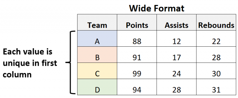
“Wide” data is organized where each variable that changes over time is in its own column and each row is a unique observation. It is probably the format you are most familiar with as it is usually easier for us to visually interpret. This is also sometimes described as “tidy” data as it’s the preferred format for data analysis, storage, and publishing. However, wide tables can be difficult to work with if they have too many columns or if the data is not well-organized. Here is a visual representation of a table in “wide” format:
Here is the same table but converted to a “long” format:
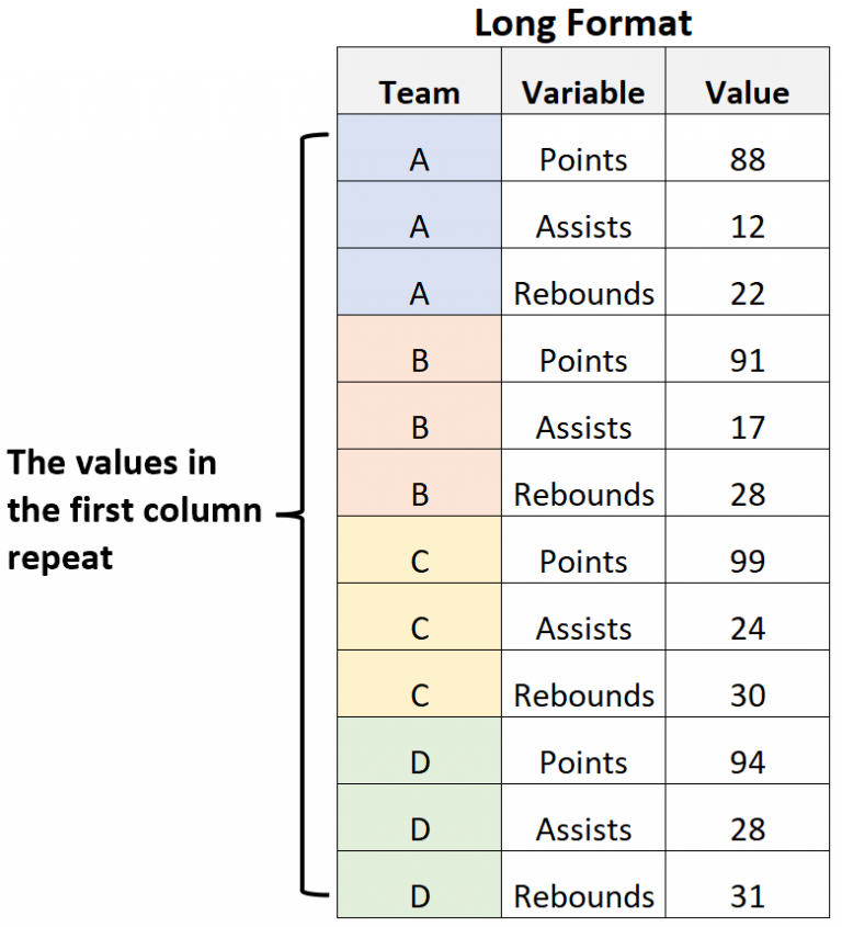
Now the values in the “Team” column repeat because each variable (Points, Assists, and Rebounds) are identified as a category in one column (Variable). Sometimes we need to reshape data into this structure if we need to visualize multiple variables in a plot or to conduct other analyses, so it is important to know how to switch between “wide” and “long” data structures. We’ll get into that in the next section.
9.3 Converting between Data Structures
For this lesson, we will continue to work with the EMP water quality data set. As a reminder, here is the structure of that data frame:
glimpse(df_wq)Rows: 62
Columns: 20
$ Station <chr> "P8", "D7", "P8", "D7", "P8", "D7", "P8", "D7", "P8…
$ Date <date> 2020-01-16, 2020-01-22, 2020-02-14, 2020-02-20, 20…
$ Chla <dbl> 0.64, 0.67, 1.46, 2.15, 1.40, 1.89, 4.73, 1.74, 6.4…
$ Pheophytin <dbl> 0.50, 0.87, 0.69, 0.50, 0.56, 1.13, 1.25, 0.89, 0.8…
$ TotAlkalinity <dbl> 98.0, 82.0, 81.0, 86.0, 80.0, 93.0, 59.0, 78.0, 63.…
$ DissAmmonia <dbl> 0.150, 0.210, 0.250, 0.140, 0.110, 0.220, 0.050, 0.…
$ DissNitrateNitrite <dbl> 2.800, 0.490, 1.700, 0.480, 1.600, 0.380, 1.070, 0.…
$ DOC <dbl> 3.90, 0.27, 2.80, 0.39, 2.00, 0.19, 2.80, 1.20, 3.1…
$ TOC <dbl> 4.10, 0.32, 2.50, 0.41, 2.10, 0.20, 2.80, 1.20, 3.1…
$ DON <dbl> NA, NA, NA, NA, NA, NA, 0.30, 0.20, 0.30, 0.10, 0.5…
$ TotPhos <dbl> 0.310, 0.082, 0.130, 0.130, 0.190, 0.100, 0.188, 0.…
$ DissOrthophos <dbl> 0.200, 0.071, 0.130, 0.065, 0.140, 0.082, 0.177, 0.…
$ TDS <dbl> 380, 9500, 340, 5800, 290, 8700, 280, 7760, 227, 11…
$ TSS <dbl> 8.9, 38.0, 2.2, 18.0, 1.4, 28.0, 6.6, 35.6, 5.3, 23…
$ TKN <dbl> 0.520, 0.480, 0.430, 0.250, 0.400, 0.200, 0.400, 0.…
$ Depth <dbl> 28.9, 18.8, 39.0, 7.1, 39.0, 7.2, 37.1, 5.2, 36.7, …
$ Secchi <dbl> 116, 30, 212, 52, 340, 48, 100, 40, 160, 44, 120, 6…
$ Microcystis <dbl> 1, 1, 1, 1, 1, 1, 3, 2, 3, 2, 4, 2, 3, 2, 2, 1, 1, …
$ SpCndSurface <dbl> 667, 15532, 647, 11369, 530, 16257, 503, 12946, 404…
$ WTSurface <dbl> 9.67, 9.97, 11.09, 12.51, 13.97, 13.81, 23.46, 21.1…We’ll start by creating a new data frame object df_wq_nutr with three common nutrients (dissolved ammonia, nitrate + nitrite, and ortho-phosphate) from the EMP water quality data set. This will allow for us to use a more condensed and simpler data frame for this example.
df_wq_nutr <- df_wq %>%
  select(Station, Date, DissAmmonia, DissNitrateNitrite, DissOrthophos)

df_wq_nutr
# A tibble: 62 × 5
Station Date DissAmmonia DissNitrateNitrite DissOrthophos
<chr> <date> <dbl> <dbl> <dbl>
1 P8 2020-01-16 0.15 2.8 0.2
2 D7 2020-01-22 0.21 0.49 0.071
3 P8 2020-02-14 0.25 1.7 0.13
4 D7 2020-02-20 0.14 0.48 0.065
5 P8 2020-03-03 0.11 1.6 0.14
6 D7 2020-03-06 0.22 0.38 0.082
7 P8 2020-06-11 0.05 1.07 0.177
8 D7 2020-06-17 0.05 0.4 0.095
9 P8 2020-07-13 0.05 0.71 0.171
10 D7 2020-07-16 0.05 0.32 0.093
# ℹ 52 more rowsPop quiz: What structure is this data frame in - “wide” or “long”?
I would describe this as “wide” format, because each nutrient parameter is in its own column and each observation (water quality sample) is in its own row. The stations (P8 and D7) repeat, but that is because EMP visited these stations each month to collect samples. Each Station and Date combination is considered a unique observation or sample.
9.3.1 “Wide” to “Long”
If we needed to reshape the data so the nutrient parameters repeat in a “Parameter” column, we could use the pivot_longer function to accomplish that:
df_wq_nutr_long <- df_wq_nutr %>%
  pivot_longer(
    cols = c(DissAmmonia, DissNitrateNitrite, DissOrthophos),
    names_to = "Parameter",
    values_to = "Value"
  )

print(df_wq_nutr_long, n = 30)
# A tibble: 186 × 4
Station Date Parameter Value
<chr> <date> <chr> <dbl>
1 P8 2020-01-16 DissAmmonia 0.15
2 P8 2020-01-16 DissNitrateNitrite 2.8
3 P8 2020-01-16 DissOrthophos 0.2
4 D7 2020-01-22 DissAmmonia 0.21
5 D7 2020-01-22 DissNitrateNitrite 0.49
6 D7 2020-01-22 DissOrthophos 0.071
7 P8 2020-02-14 DissAmmonia 0.25
8 P8 2020-02-14 DissNitrateNitrite 1.7
9 P8 2020-02-14 DissOrthophos 0.13
10 D7 2020-02-20 DissAmmonia 0.14
11 D7 2020-02-20 DissNitrateNitrite 0.48
12 D7 2020-02-20 DissOrthophos 0.065
13 P8 2020-03-03 DissAmmonia 0.11
14 P8 2020-03-03 DissNitrateNitrite 1.6
15 P8 2020-03-03 DissOrthophos 0.14
16 D7 2020-03-06 DissAmmonia 0.22
17 D7 2020-03-06 DissNitrateNitrite 0.38
18 D7 2020-03-06 DissOrthophos 0.082
19 P8 2020-06-11 DissAmmonia 0.05
20 P8 2020-06-11 DissNitrateNitrite 1.07
21 P8 2020-06-11 DissOrthophos 0.177
22 D7 2020-06-17 DissAmmonia 0.05
23 D7 2020-06-17 DissNitrateNitrite 0.4
24 D7 2020-06-17 DissOrthophos 0.095
25 P8 2020-07-13 DissAmmonia 0.05
26 P8 2020-07-13 DissNitrateNitrite 0.71
27 P8 2020-07-13 DissOrthophos 0.171
28 D7 2020-07-16 DissAmmonia 0.05
29 D7 2020-07-16 DissNitrateNitrite 0.32
30 D7 2020-07-16 DissOrthophos 0.093
# ℹ 156 more rowsNow you can see that the nutrient parameters repeat in a “Parameter” column and the data values are now in the “Value” column. Let’s take a closer look on how to use the pivot_longer function. The three necessary arguments in this function (after the first argument which is the data frame itself) are:
-
colsdefines which columns are to be moved into one column. -
names_tonames the variable to move the columns incolsto. -
values_tonames the variable to move the cell values of the columns incolsto.
Note
Note that the variables in both names_to and values_to require “quotes” since we are creating new columns.
9.3.2 “Long” to “Wide”
Now, imagine that we wanted to reshape the df_wq_nutr_long data frame that we just created back into its original “wide” structure. We could just use the original data frame df_wq_nutr, but let’s assume that we don’t have that. In this case we could use the pivot_wider function:
df_wq_nutr_wide <- df_wq_nutr_long %>%
  pivot_wider(names_from = Parameter, values_from = Value)

df_wq_nutr_wide
# A tibble: 62 × 5
Station Date DissAmmonia DissNitrateNitrite DissOrthophos
<chr> <date> <dbl> <dbl> <dbl>
1 P8 2020-01-16 0.15 2.8 0.2
2 D7 2020-01-22 0.21 0.49 0.071
3 P8 2020-02-14 0.25 1.7 0.13
4 D7 2020-02-20 0.14 0.48 0.065
5 P8 2020-03-03 0.11 1.6 0.14
6 D7 2020-03-06 0.22 0.38 0.082
7 P8 2020-06-11 0.05 1.07 0.177
8 D7 2020-06-17 0.05 0.4 0.095
9 P8 2020-07-13 0.05 0.71 0.171
10 D7 2020-07-16 0.05 0.32 0.093
# ℹ 52 more rowsThe resulting df_wq_nutr_wide data frame is back in the original “wide” structure that we started with. Again, let’s review how to use the pivot_wider function. This function has two necessary arguments after the first one for the data frame:
-
names_fromdefines the column from which the new column names will be named to. -
values_fromdefines the column from which the cell values will be derived from.
Note
Note that the variables in both names_from and values_from are unquoted since we’re defining existing columns.
9.3.3 Exercise
Now its your turn to try out the reshaping functions we just learned about.
Use
pivot_longerto create a data frame fromdf_wqwhere the water quality measurements (“Secchi”, “SpCndSurface”, and “WTSurface”) are reshaped into a column named “WQ_Measurement” and their values are in a column called “Result”. Assign this data frame to a new object to be used later.
HINT: Make sure to useselectto subset the data frame to contain the columns you need. Use our nutrient example above.Now, use
pivot_widerto reshape the “long” data frame you created in #1 back to its original “wide” structure.
Click below for the answer when you are done!
Code
# Create new "long" data frame for just the water quality measurements
df_wq_meas_long <- df_wq %>%
  select(Station, Date, Secchi, SpCndSurface, WTSurface) %>%
  pivot_longer(
    cols = c(Secchi, SpCndSurface, WTSurface),
    names_to = "WQ_Measurement",
    values_to = "Result"
  )

# Take a look at df_wq_meas_long
df_wq_meas_long

# Reshape df_wq_meas_long back to it's original "Wide" structure
df_wq_meas_long %>% pivot_wider(names_from = WQ_Measurement, values_from = Result)