Basic Stats
fish_yolo_url <- "https://portal.edirepository.org/nis/dataviewer?packageid=edi.233.2&entityid=015e494911cf35c90089ced5a3127334"
fish_data <- readr::read_csv(fish_yolo_url)
str(fish_data)
## spec_tbl_df [182,414 x 32] (S3: spec_tbl_df/tbl_df/tbl/data.frame)
##  $ SampleDate          : chr [1:182414] "1/16/1998" "1/16/1998" "1/19/1998" "1/19/1998" ...
##  $ SampleTime          : 'hms' num [1:182414] 14:05:00 15:00:00 12:17:00 12:17:00 ...
##   ..- attr(*, "units")= chr "secs"
##  $ StationCode         : chr [1:182414] "YB" "YB" "YB" "YB" ...
##  $ MethodCode          : chr [1:182414] "BSEIN" "BSEIN" "FNET" "FNET" ...
##  $ GearID              : chr [1:182414] "SEIN50" "SEIN50" "FKNT" "FKNT" ...
##  $ CommonName          : chr [1:182414] "Threadfin Shad" "Inland Silverside" "Threadfin Shad" "Chinook Salmon" ...
##  $ GeneticallyConfirmed: chr [1:182414] "No" "No" "No" "No" ...
##  $ GeneticID           : logi [1:182414] NA NA NA NA NA NA ...
##  $ Field_ID_CommonName : chr [1:182414] "Threadfin Shad" "Inland Silverside" "Threadfin Shad" "Chinook Salmon" ...
##  $ ForkLength          : num [1:182414] 90 73 88 38 71 62 58 50 81 49 ...
##  $ Count               : num [1:182414] 1 1 1 1 1 1 1 1 1 1 ...
##  $ FishSex             : chr [1:182414] NA NA NA NA ...
##  $ Race                : chr [1:182414] "n/p" "n/p" "n/p" "n/p" ...
##  $ MarkCode            : chr [1:182414] "n/p" "n/p" "n/p" "n/p" ...
##  $ CWTSample           : logi [1:182414] FALSE FALSE FALSE FALSE FALSE FALSE ...
##  $ FishTagID           : chr [1:182414] NA NA NA NA ...
##  $ StageCode           : chr [1:182414] "n/p" "n/p" "n/p" "CHN_P" ...
##  $ Dead                : chr [1:182414] "No" "No" "No" "No" ...
##  $ GearConditionCode   : num [1:182414] 3 3 1 1 1 1 1 1 1 1 ...
##  $ WeatherCode         : chr [1:182414] "CLD" "CLD" "RAN" "RAN" ...
##  $ WaterTemperature    : num [1:182414] 11.7 11.7 11.1 11.1 11.1 ...
##  $ Secchi              : num [1:182414] NA NA 0.16 0.16 0.07 ...
##  $ Conductivity        : num [1:182414] NA NA NA NA NA NA NA NA NA NA ...
##  $ SpCnd               : num [1:182414] NA NA NA NA NA NA NA NA NA NA ...
##  $ DO                  : num [1:182414] NA NA NA NA NA NA NA NA NA NA ...
##  $ pH                  : num [1:182414] NA NA NA NA NA NA NA NA NA NA ...
##  $ Turbidity           : num [1:182414] NA NA NA NA NA NA NA NA NA NA ...
##  $ SubstrateCode       : chr [1:182414] "VG" "MD" NA NA ...
##  $ Tide                : chr [1:182414] NA NA NA NA ...
##  $ VolumeSeined        : num [1:182414] NA NA NA NA NA NA NA NA NA NA ...
##  $ Latitude            : num [1:182414] 38.6 38.6 NA NA NA ...
##  $ Longitude           : num [1:182414] -122 -122 NA NA NA ...
##  - attr(*, "spec")=
##   .. cols(
##   ..   SampleDate = col_character(),
##   ..   SampleTime = col_time(format = ""),
##   ..   StationCode = col_character(),
##   ..   MethodCode = col_character(),
##   ..   GearID = col_character(),
##   ..   CommonName = col_character(),
##   ..   GeneticallyConfirmed = col_character(),
##   ..   GeneticID = col_logical(),
##   ..   Field_ID_CommonName = col_character(),
##   ..   ForkLength = col_double(),
##   ..   Count = col_double(),
##   ..   FishSex = col_character(),
##   ..   Race = col_character(),
##   ..   MarkCode = col_character(),
##   ..   CWTSample = col_logical(),
##   ..   FishTagID = col_character(),
##   ..   StageCode = col_character(),
##   ..   Dead = col_character(),
##   ..   GearConditionCode = col_double(),
##   ..   WeatherCode = col_character(),
##   ..   WaterTemperature = col_double(),
##   ..   Secchi = col_double(),
##   ..   Conductivity = col_double(),
##   ..   SpCnd = col_double(),
##   ..   DO = col_double(),
##   ..   pH = col_double(),
##   ..   Turbidity = col_double(),
##   ..   SubstrateCode = col_character(),
##   ..   Tide = col_character(),
##   ..   VolumeSeined = col_double(),
##   ..   Latitude = col_double(),
##   ..   Longitude = col_double()
##   .. )
##  - attr(*, "problems")=<externalptr>
fish_lmb <- fish_data %>% filter(CommonName == "Largemouth Bass")
fish_lmb2 <- fish_lmb %>% filter(MethodCode %in% c("BSEIN", "RSTR"))
Parametric Stats
T-test
### 1. Independent-samples t-test: Is there a difference in LMB Count by Method? ----------------
(lmb.ttest <- t.test(fish_lmb2$Count~fish_lmb2$MethodCode)) # not significant
##
##  Welch Two Sample t-test
##
## data:  fish_lmb2$Count by fish_lmb2$MethodCode
## t = -2.4938, df = 372.14, p-value = 0.01307
## alternative hypothesis: true difference in means between group BSEIN and group RSTR is not equal to 0
## 95 percent confidence interval:
##  -1.6055186 -0.1898624
## sample estimates:
## mean in group BSEIN  mean in group RSTR
##            1.146387            2.044077
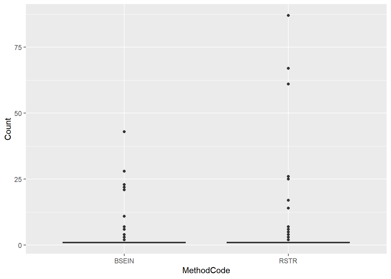
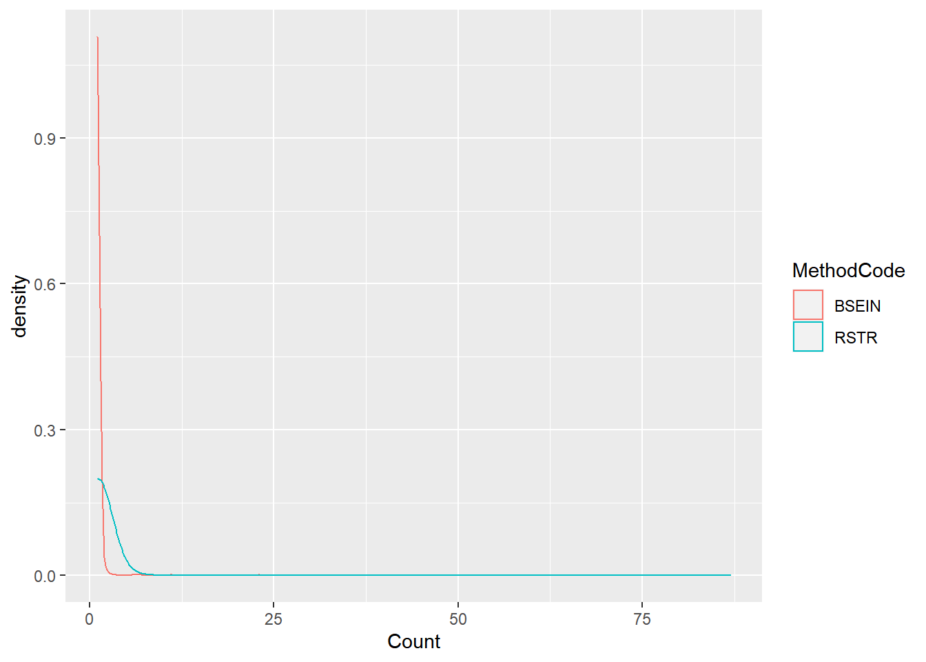
# Plot
ggplot(fish_lmb2, aes(x = MethodCode, y = Count)) + geom_boxplot()
ggplot(fish_lmb2, aes(x = Count, color = MethodCode)) + geom_density()
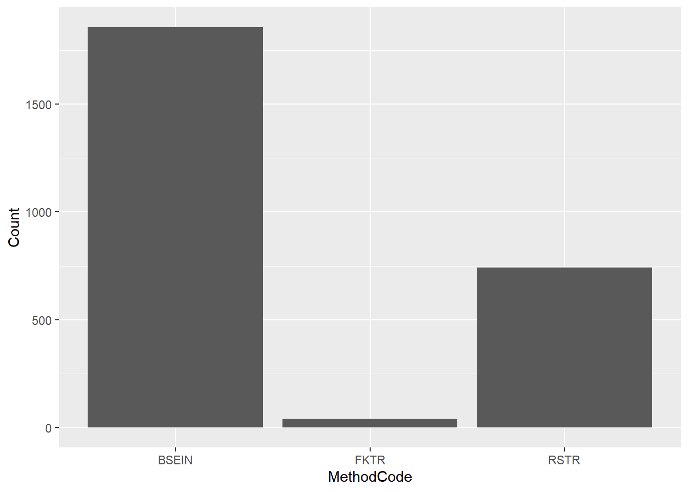
ggplot(fish_lmb, aes(x = MethodCode, y = Count)) + geom_col() # This works best for data with lots of zeros
### 2. Paired t-test: Does a treatment cause a difference? Did Action Phase alter Count of LMB? -------------
(lmb.ttest2 <- t.test(fish_lmb2$Count ~ fish_lmb2$MethodCode)) # significant
##
##  Welch Two Sample t-test
##
## data:  fish_lmb2$Count by fish_lmb2$MethodCode
## t = -2.4938, df = 372.14, p-value = 0.01307
## alternative hypothesis: true difference in means between group BSEIN and group RSTR is not equal to 0
## 95 percent confidence interval:
##  -1.6055186 -0.1898624
## sample estimates:
## mean in group BSEIN  mean in group RSTR
##            1.146387            2.044077
# Plot: Figure out the direction of the trend
# ggplot(fish_lmb2, aes(x = ActionPhase, y = Count)) + geom_boxplot()
# ggplot(fish_lmb2, aes(x = Count, color = ActionPhase)) + geom_density()
# ggplot(fish_lmb2, aes(x = ActionPhase, y = Count)) + geom_col() # This works best for data with lots of zeros

### 3. One-sample t-test: Is the Count greater than 0? ---------------------------------------
(lmb.ttest3 <- t.test(fish_lmb2$Count, mu = 0)) # p < 0.05, Yes, it is
##
##  One Sample t-test
##
## data:  fish_lmb2$Count
## t = 17.633, df = 1981, p-value < 2.2e-16
## alternative hypothesis: true mean is not equal to 0
## 95 percent confidence interval:
##  1.165012 1.456583
## sample estimates:
## mean of x
##  1.310797
Non-parametric Statistics