Chapter 6 Spatial data and making maps
We will cover: 1. Basics of using sf package, converting lat/lon to a spatial data frame. 2. Importing shapefiles 3. Making a map of your lats/lons 4. Add inset map 5. Add scale bar, north arrow, labels 6. Add basemap 7. Writing map image and map files
Packages
library(ggplot2)
library(dplyr)
library(sf)
library(viridis)
6.1 Load data
Latitude/Longitude data from IEP zooplankton data
# Latitude/Longitude data
stations_URL <- "https://portal.edirepository.org/nis/dataviewer?packageid=edi.539.3&entityid=343cb43b41eb112ac36b605f1cff1f92"

# Create a fake n variable to have something to plot.
stations <- readr::read_csv(stations_URL) %>%
  mutate(n = round(runif(n = 1:nrow(.), min = 1, max = 100),0)) %>%
  mutate(Source = factor(Source)) %>%
  filter(!is.na(Latitude))

dplyr::glimpse(stations)
## Rows: 368
## Columns: 5
## $ Source <fct> EMP, EMP, EMP, EMP, EMP, EMP, EMP, EMP, EMP, EMP, EMP, EMP, ~
## $ Station <chr> "NZ002", "NZ003", "NZ004", "NZ005", "NZ020", "NZ022", "NZ024~
## $ Latitude <dbl> 38.06028, 38.05250, 38.02917, 38.03167, 38.05972, 38.07194, ~
## $ Longitude <dbl> -122.2069, -122.1783, -122.1583, -122.1353, -122.1097, -122.~
## $ n <dbl> 63, 63, 46, 80, 66, 81, 47, 92, 22, 21, 85, 51, 12, 5, 54, 9~# create a subset of stations
stationlist_filt <- sample_n(stations, 20) %>% select(Station)
stationlist_filt <- stationlist_filt$StationShapefiles
# Delta waterways
library(deltamapr)
plot(WW_Delta)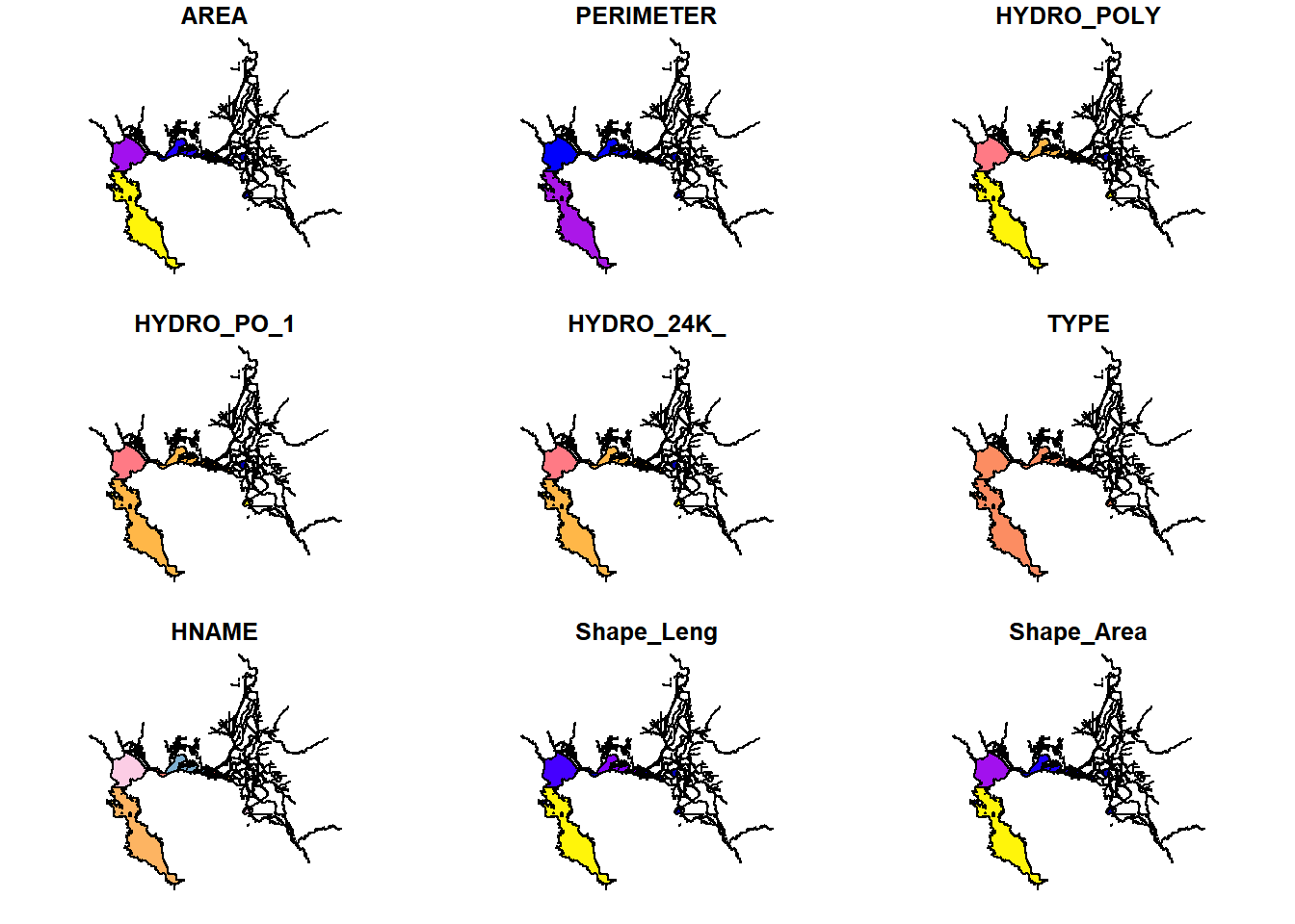
glimpse(WW_Delta)## Rows: 282
## Columns: 10
## $ AREA <dbl> 73544304.00, 87637.30, 7915130.00, 103906.00, 106371.00, 15~
## $ PERIMETER <dbl> 1033340.000, 3319.230, 87427.898, 2718.730, 2798.310, 3391.~
## $ HYDRO_POLY <int> 791, 1965, 1967, 1970, 1977, 1982, 1992, 2001, 2006, 2008, ~
## $ HYDRO_PO_1 <int> 797, 1963, 1965, 1969, 1974, 1978, 1989, 2008, 2012, 2011, ~
## $ HYDRO_24K_ <int> 798, 1964, 1966, 1970, 1975, 1979, 1990, 2009, 2013, 2012, ~
## $ TYPE <chr> "MR", "S", "C", "L", "L", "S", "S", "MR", "MR", "MR", "MR",~
## $ HNAME <chr> "SACRAMENTO RIVER", "W", "SACTO. R DEEP WATER SH CHAN", "GR~
## $ Shape_Leng <dbl> 2.448454165, 0.035719722, 0.828813375, 0.026377690, 0.02830~
## $ Shape_Area <dbl> 3.476418e-03, 9.063090e-06, 8.166341e-04, 1.074391e-05, 1.0~
## $ geometry <POLYGON [°]> POLYGON ((-121.5099 38.2471..., POLYGON ((-121.5673~# Regions
Regions <- deltamapr::R_EDSM_Subregions_Mahardja_FLOAT
plot(Regions)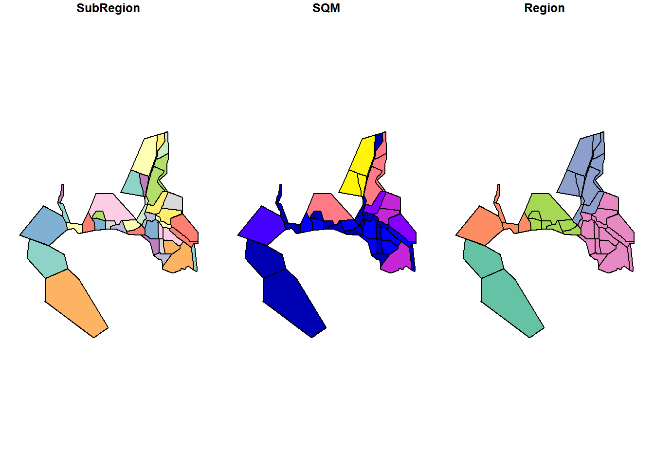
glimpse(Regions)## Rows: 40
## Columns: 4
## $ SubRegion <chr> "Cache Slough and Lindsey Slough", "Carquinez Strait", "Conf~
## $ SQM <dbl> 471689278, 48215634, 39171738, 182085789, 94761329, 23726124~
## $ Region <chr> "North", "Far West", "West", "South", "South", "South", "Wes~
## $ geometry <POLYGON [m]> POLYGON ((611964 4246976, 6..., POLYGON ((567190.8 4~# States
library(USAboundaries)
California_sf <- us_states(states = "California")
plot(California_sf[1])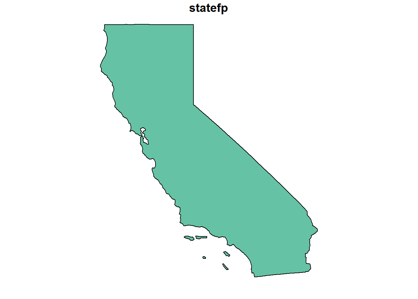
6.2 Get data into spatial form
# Define the projection of your points, usually WGS 84 (= crs 4326)
stations_sf <- st_as_sf(stations, coords = c("Longitude", "Latitude"), crs = 4326)

# Look at shapefile
head(stations_sf)
## Simple feature collection with 6 features and 3 fields
## Geometry type: POINT
## Dimension: XY
## Bounding box: xmin: -122.2069 ymin: 38.02917 xmax: -122.0961 ymax: 38.07194
## Geodetic CRS: WGS 84
## # A tibble: 6 x 4
## Source Station n geometry
## <fct> <chr> <dbl> <POINT [°]>
## 1 EMP NZ002 63 (-122.2069 38.06028)
## 2 EMP NZ003 63 (-122.1783 38.0525)
## 3 EMP NZ004 46 (-122.1583 38.02917)
## 4 EMP NZ005 80 (-122.1353 38.03167)
## 5 EMP NZ020 66 (-122.1097 38.05972)
## 6 EMP NZ022 81 (-122.0961 38.07194)plot(stations_sf$geometry)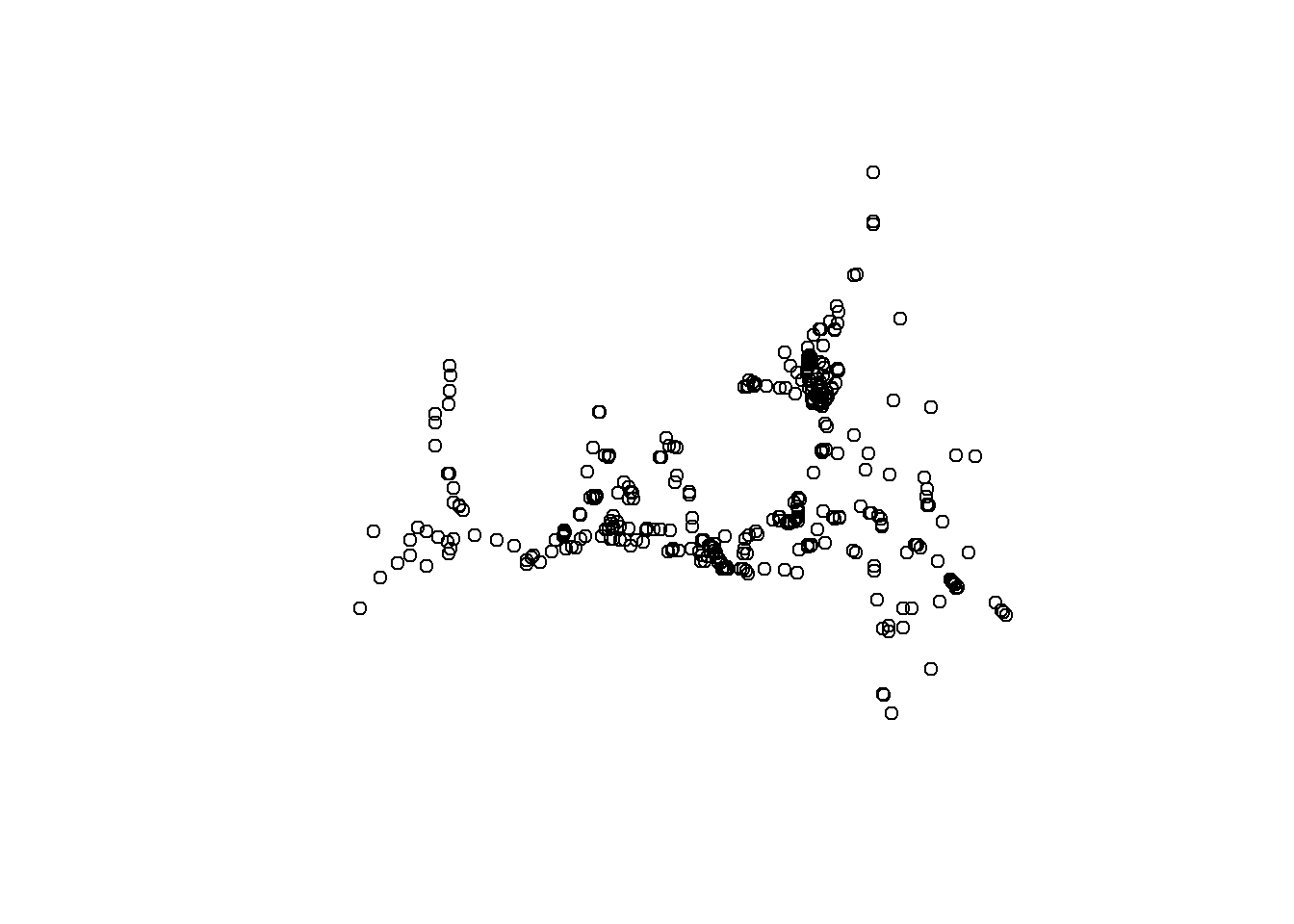
plot(stations_sf)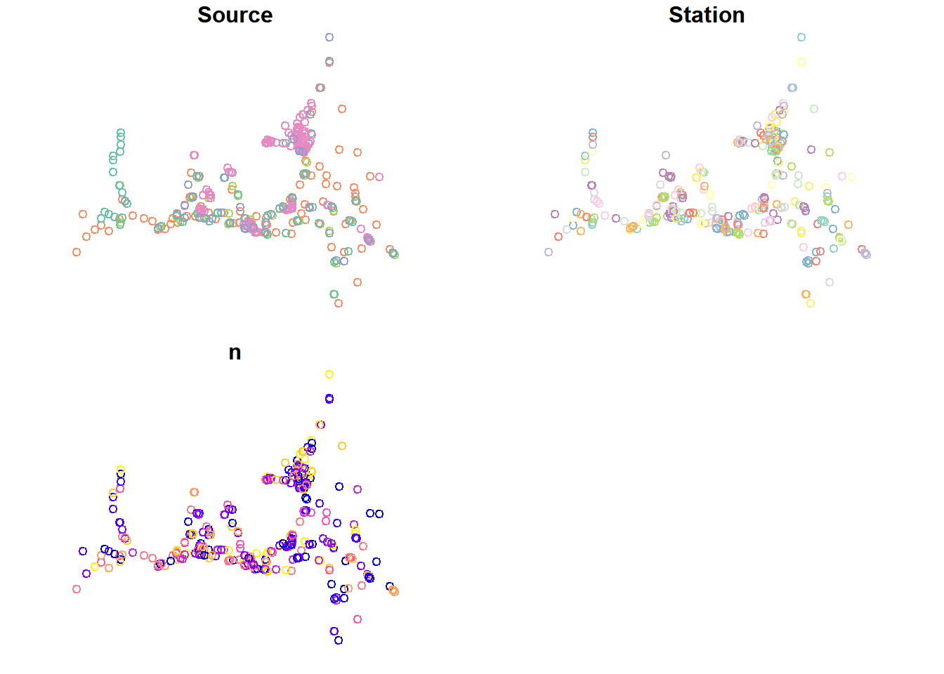
6.2.1 Spatial projections
You want to make sure all your different files are in the same projection, or they will look mis-aligned.
st_crs(WW_Delta) # In 4269## Coordinate Reference System:
## User input: NAD83
## wkt:
## GEOGCRS["NAD83",
## DATUM["North American Datum 1983",
## ELLIPSOID["GRS 1980",6378137,298.257222101,
## LENGTHUNIT["metre",1]]],
## PRIMEM["Greenwich",0,
## ANGLEUNIT["degree",0.0174532925199433]],
## CS[ellipsoidal,2],
## AXIS["latitude",north,
## ORDER[1],
## ANGLEUNIT["degree",0.0174532925199433]],
## AXIS["longitude",east,
## ORDER[2],
## ANGLEUNIT["degree",0.0174532925199433]],
## ID["EPSG",4269]]st_crs(stations_sf) # In 4326## Coordinate Reference System:
## User input: EPSG:4326
## wkt:
## GEOGCRS["WGS 84",
## DATUM["World Geodetic System 1984",
## ELLIPSOID["WGS 84",6378137,298.257223563,
## LENGTHUNIT["metre",1]]],
## PRIMEM["Greenwich",0,
## ANGLEUNIT["degree",0.0174532925199433]],
## CS[ellipsoidal,2],
## AXIS["geodetic latitude (Lat)",north,
## ORDER[1],
## ANGLEUNIT["degree",0.0174532925199433]],
## AXIS["geodetic longitude (Lon)",east,
## ORDER[2],
## ANGLEUNIT["degree",0.0174532925199433]],
## USAGE[
## SCOPE["Horizontal component of 3D system."],
## AREA["World."],
## BBOX[-90,-180,90,180]],
## ID["EPSG",4326]]st_crs(California_sf) # In 4326## Coordinate Reference System:
## User input: EPSG:4326
## wkt:
## GEOGCRS["WGS 84",
## DATUM["World Geodetic System 1984",
## ELLIPSOID["WGS 84",6378137,298.257223563,
## LENGTHUNIT["metre",1]]],
## PRIMEM["Greenwich",0,
## ANGLEUNIT["degree",0.0174532925199433]],
## CS[ellipsoidal,2],
## AXIS["geodetic latitude (Lat)",north,
## ORDER[1],
## ANGLEUNIT["degree",0.0174532925199433]],
## AXIS["geodetic longitude (Lon)",east,
## ORDER[2],
## ANGLEUNIT["degree",0.0174532925199433]],
## USAGE[
## SCOPE["Horizontal component of 3D system."],
## AREA["World."],
## BBOX[-90,-180,90,180]],
## ID["EPSG",4326]]stations_4269 <- st_transform(stations_sf, crs = 4269)
california_4269 <- st_transform(California_sf, crs = 4269)6.3 Basic Spatial Operations
Assign points to regions
Nearest neighbor
Intersections
6.4 Make maps
6.4.1 Basic maps
Color by Monitoring Program
ggplot() +
    geom_sf(data = WW_Delta) +
    geom_sf(data = stations_4269, aes(fill = Source), shape = 21) +
    scale_fill_viridis(discrete = TRUE) +
    ggtitle("Number of Zooplankton Samples by Station") +
    theme_bw()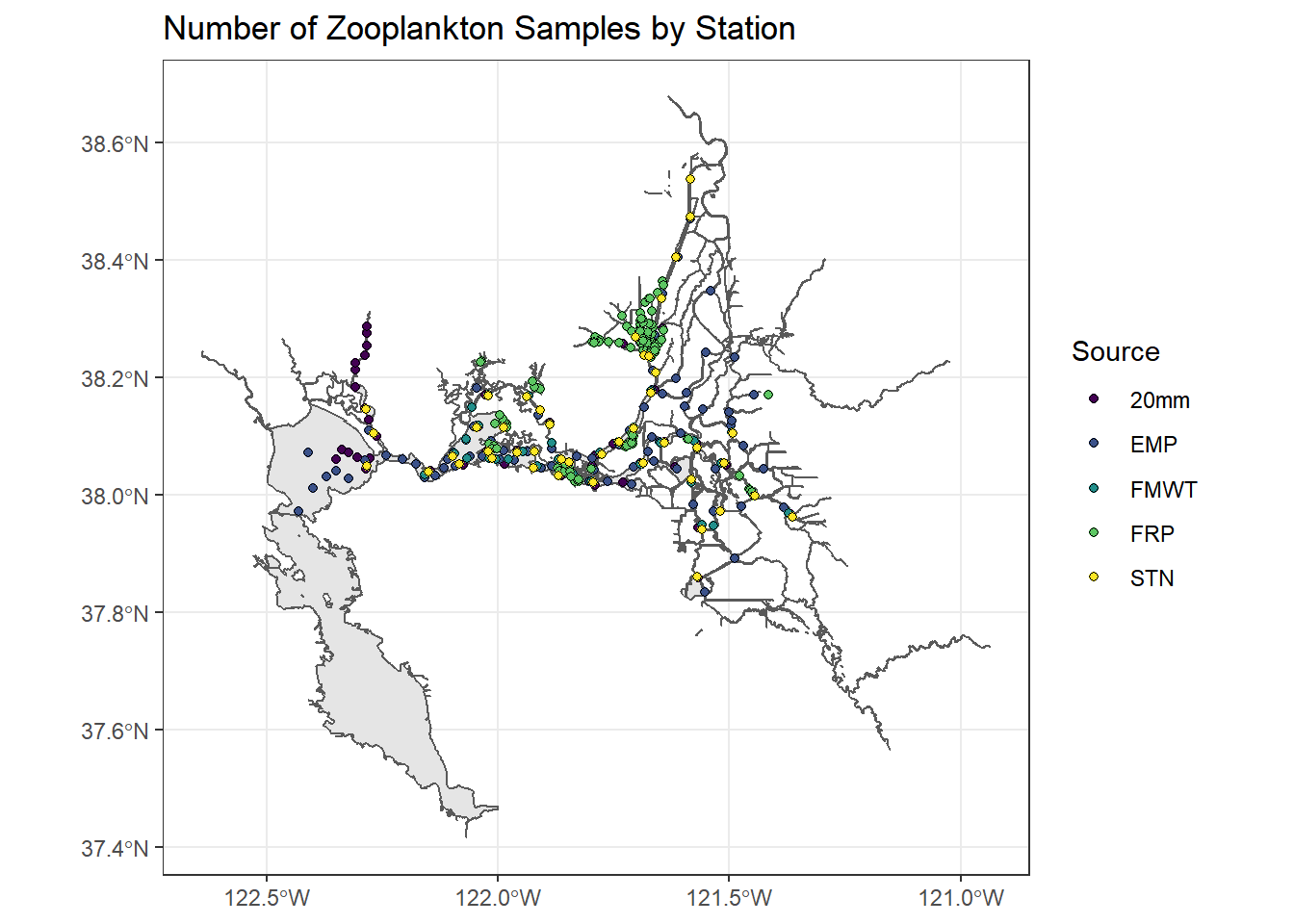
You can also modify the size of the points by size
# Making a smaller dataset
stations_filtered_4269 <- stations_4269 %>%
  filter(Station %in% stationlist_filt)

(simplemap <- ggplot() +
    geom_sf(data = WW_Delta, fill = "lightblue", color = "lightblue") +
    geom_sf(data = stations_filtered_4269, aes(fill = Source, size = n), shape = 21, alpha = 0.7) +
    scale_fill_viridis(discrete = TRUE, option = "plasma") +
    scale_size_continuous(range = c(0,3)) +
    ggtitle("Number of Zooplankton Samples by Station") +
    theme_bw())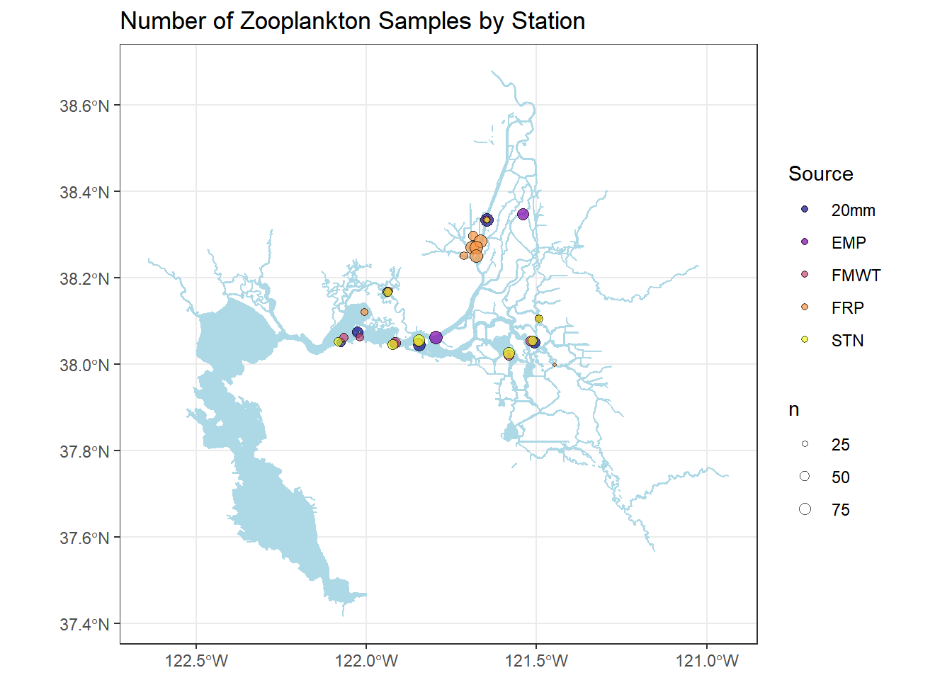
You can add region delineations as well
ggplot() +
    geom_sf(data = WW_Delta, fill = "lightblue", color = "lightblue") +
    geom_sf(data = Regions, aes(color = Region), alpha = 0.3) +
    geom_sf(data = stations_filtered_4269, aes(fill = Source, size = n), shape = 21) +
    scale_fill_viridis(discrete = TRUE, option = "plasma") +
  scale_color_viridis(discrete = TRUE, option = "turbo") +
    scale_size_continuous(range = c(0,3)) +
    ggtitle("Number of Zooplankton Samples by Station") +
    theme_bw()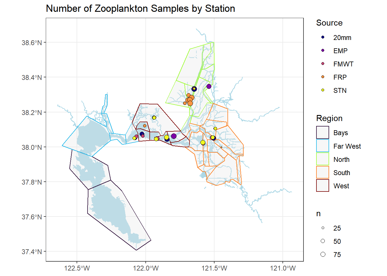
6.4.2 Add arrows and scale bars, dotted lines
require(ggspatial)
# https://www.r-spatial.org/r/2018/10/25/ggplot2-sf.html

(simplemap2 <- simplemap +
  annotation_north_arrow(location = "tr", which_north = "true",
        pad_x = unit(0.1, "in"), pad_y = unit(0.1, "in"),
        style = north_arrow_fancy_orienteering) +
  annotation_scale(location = "bl", bar_cols = c("pink", "white", "pink", "white")) +
  theme(axis.title = element_blank(),
        panel.grid.major = element_line(color = "grey80", linetype = "dashed", size = 0.5)))
6.4.3 Add labels to map
# Adding text
simplemap2 +
  geom_text(data = filter(stations, Station %in% stationlist_filt), aes(x = Longitude, y = Latitude, label = Station), size = 2, check_overlap = FALSE, color = "darkblue", nudge_x = 0.02, nudge_y = 0.02) +
annotate(geom = "text", x = -122.4, y = 37.85, label = "San Francisco Bay", fontface = "italic", color = "grey22", size = 3.5 ) 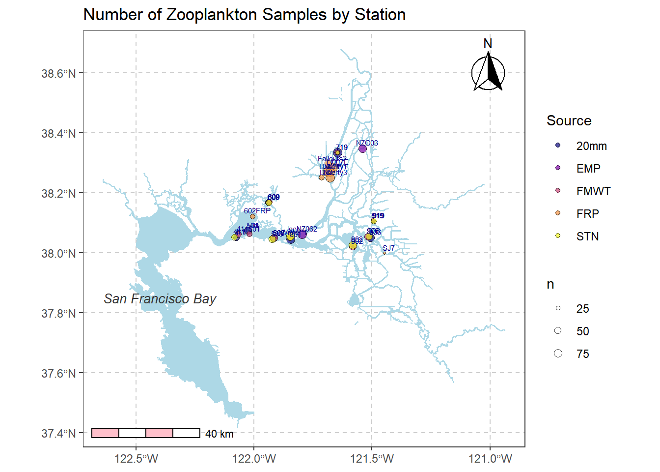
6.4.4 Add inset map
# Figure out boundary box for your stations; perhaps add a small buffer
insetbbox0 = st_as_sfc(st_bbox(WW_Delta))
insetbbox = st_buffer(insetbbox0, 0.2)

(inset <- ggplot() +
  geom_sf(data = california_4269, fill = "white") +
  geom_sf(data = insetbbox0, fill = NA, color = "red", size = 0.5) +
  theme_void())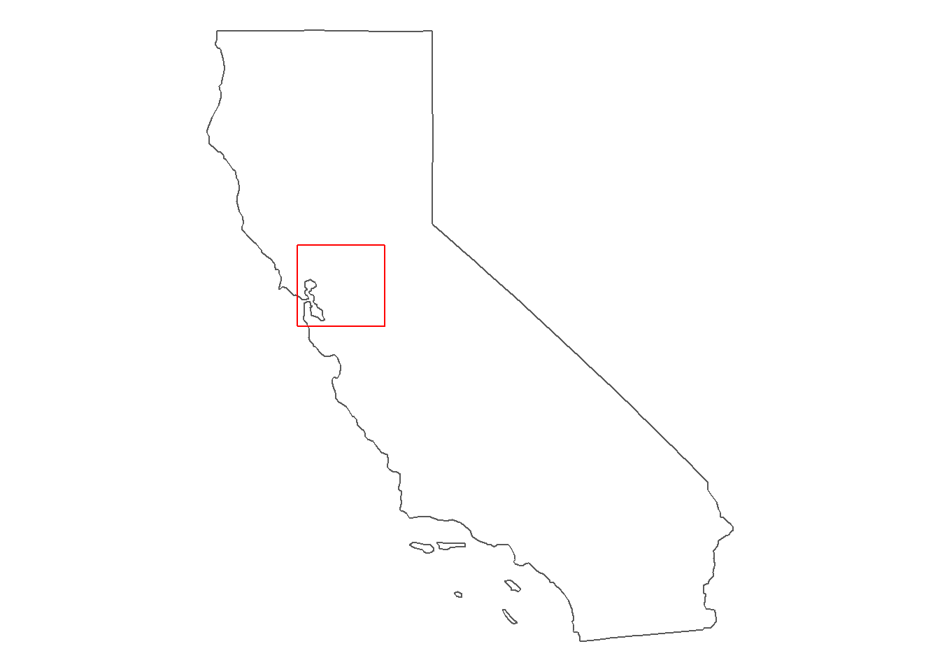
Combine main map with inset map
Will need to play with where you want the inset to be so as not to overlap with your map
library(cowplot)
inset_map = ggdraw() +
  draw_plot(simplemap2) +
  draw_plot(inset, x = 0.15, y = 0.63, width = 0.3, height = 0.3)

inset_map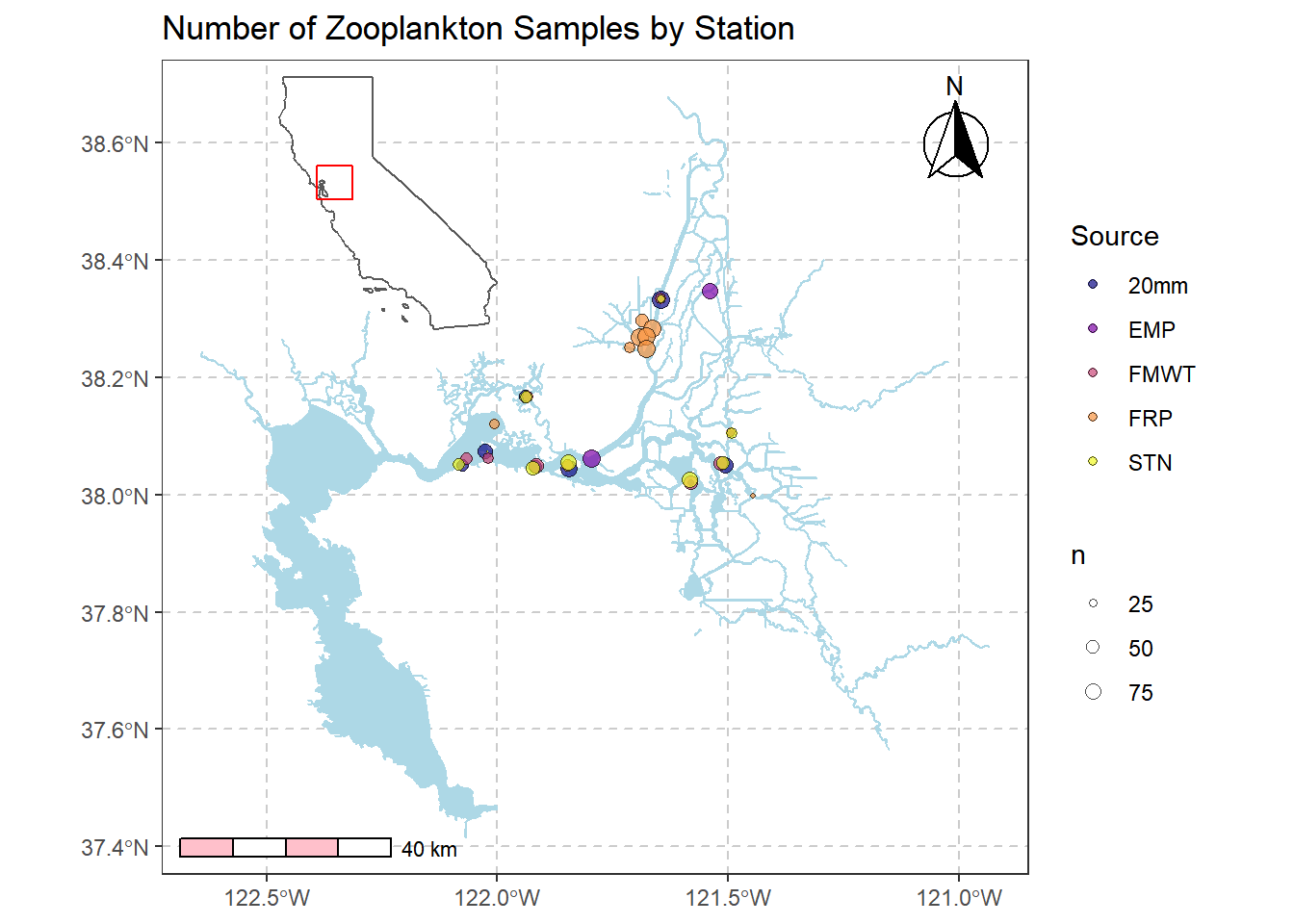
6.5 Basemaps
Download basemaps from get_stamenmap
library(ggmap)Define coordinate bounding box. You could also use lat/lon if you want.
buffer = 0.2
coordDict = list(
    'minLat' = min(stations$Latitude) - buffer,
    'maxLat' = max(stations$Latitude) -0.1,
    'minLon' = min(stations$Longitude) - buffer,
    'maxLon' = max(stations$Longitude) + buffer
)

# Create map object using your bounded coordinates
map_obj <- get_stamenmap(
  bbox = c(left = coordDict[['minLon']], bottom = coordDict[['minLat']], right = coordDict[['maxLon']], top = coordDict[['maxLat']]), # the bounding box
  zoom = 9, # zoom lvl; higher number = more detail (but also more processing power)
  maptype = 'terrain-background'# type of basemap; 'terrain' is my default, but check help(get_stamenmap) for a full list
  )
Plot your basemap
# Plot the map
map <- ggmap(map_obj, legend = "right")
map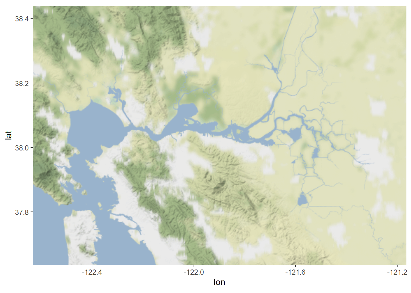
Add basemap to earlier map.
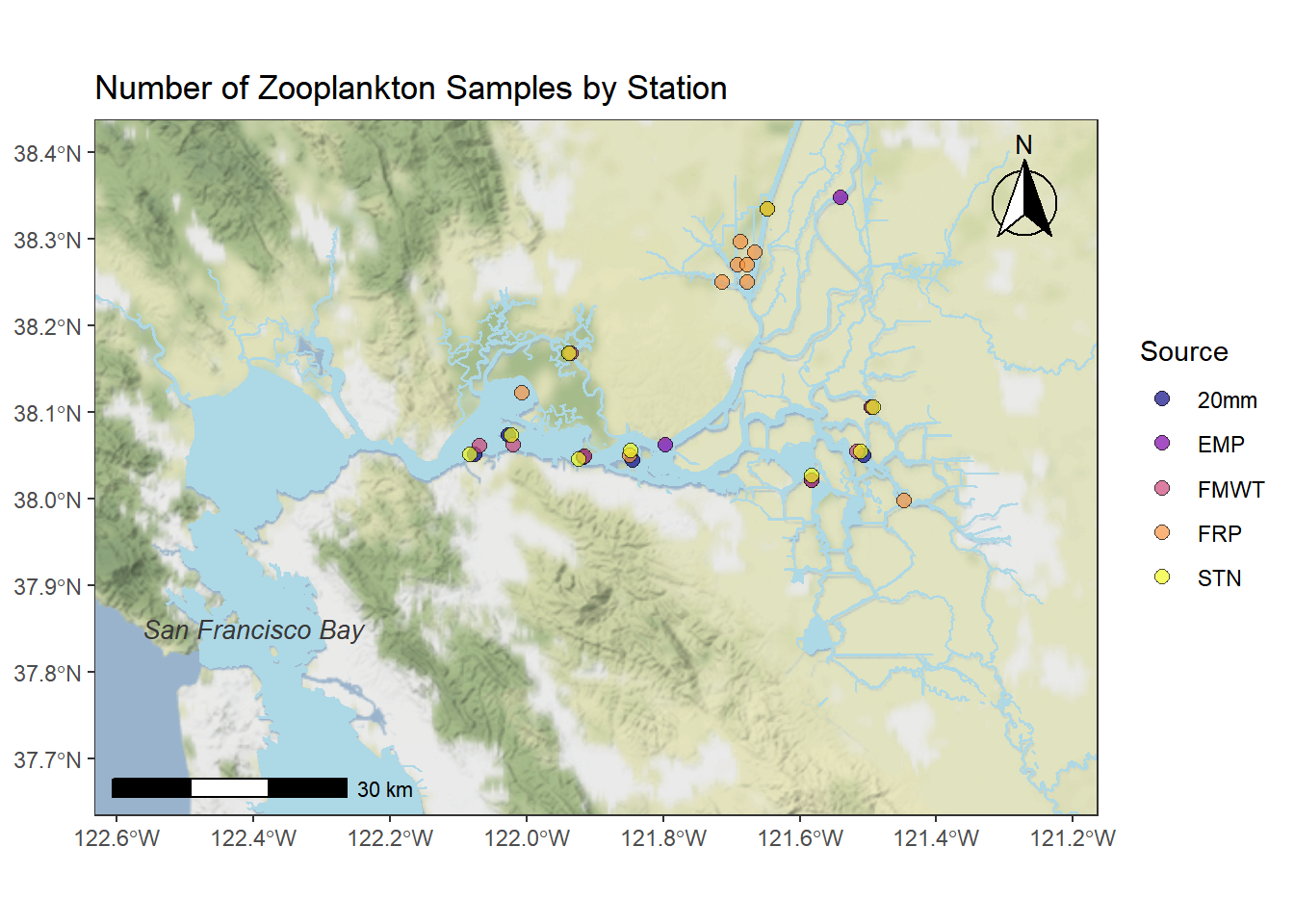
map2 <- ggmap(map_obj) +
    geom_sf(data = WW_Delta, fill = "lightblue", color = "lightblue", inherit.aes = FALSE) +
    geom_sf(data = stations_filtered_4269, aes(fill = Source), shape = 21, alpha = 0.7, size = 2.5, inherit.aes = FALSE) +
 annotate(geom = "text", x = -122.4, y = 37.85, label = "San Francisco Bay", fontface = "italic", color = "grey22", size = 3.5 ) +
  annotation_north_arrow(location = "tr", which_north = "true",
        pad_x = unit(0.1, "in"), pad_y = unit(0.1, "in"),
        style = north_arrow_fancy_orienteering) +
  annotation_scale(location = "bl", bar_cols = c("black", "white", "black", "white")) +
    scale_fill_viridis(discrete = TRUE, option = "plasma") +
    ggtitle("Number of Zooplankton Samples by Station") +
    theme_bw()+ theme(axis.title = element_blank(),
        panel.grid.major = element_line(color = "grey80", linetype = "dashed", size = 0.5))
map2